
Evapotranspiration Trends and Interactions in Light of the Anthropogenic Footprint and the Climate Crisis: A Review


Department of Geology, University of Patras, 26504 Rion, Greece
*
Author to whom correspondence should be addressed.
Hydrology 2021, 8(4), 163; https://doi.org/10.3390/hydrology8040163
Submission received: 16 September 2021
/
Revised: 7 October 2021
/
Accepted: 27 October 2021
/
Published: 1 November 2021
(This article belongs to the Special Issue Advances in Evaporation and Evaporative Demand)
Abstract
:Evapotranspiration (ET) is a parameter of major importance participating in both hydrological cycle and surface energy balance. Trends of ET are discussed along with the dependence of evaporation to key environmental variables. The evaporation paradox can be approached via natural phenomena aggravated by anthropogenic impact. ET appears as one of the most affected parameters by human activities. Complex hydrological processes are governed by local environmental conditions thus generalizations are difficult. However, in some settings, common hydrological interactions could be detected. Mediterranean climate regions (MCRs) appear vulnerability to the foreseen increase in ET, aggravated by precipitation shifting and air temperature warming, whereas in tropical forests its role is rather beneficial. ET determines groundwater level and quality. Groundwater level appeared to be a robust predictor of annual ET for peatlands in Southeast Asia. In semi-arid to arid areas, increases in ET have implications on water availability and soil salinization. ET-changes after a wildfire can be substantial for groundwater recharge if a canopy-loss threshold is surpassed. Those consequences are site-specific. Post-fire ET rebound seems climate and fire-severity-dependent. Overall, this qualitative structured review sets the foundations for interdisciplinary researchers and water managers to deploy ET as a means to address challenging environmental issues such as water availability.
1. Introduction
The importance of evapotranspiration (ET) is demonstrated by its participation in the hydrological cycle (as a hydrological process) and in the surface energy balance (as a flux) [1]. Taking into account that a high percentage of the precipitated water is evaporated and transpired (e.g., 65% Ireland [2]; 62% Greece [3]) it is obvious that water budgets are dictated by the fluctuations of ET and subsequently by the dependency of ET on several environmental parameters [4,5,6]. ET according to researchers is a component that is not perfectly understood yet. Thus, it should be thoroughly studied as a major key parameter involving numerous mechanisms, mediating fluctuations of other variables, and controlling processes or causing considerable problems after intense disturbances by human activity or climate change.
1.1. Types of ET
Actual evapotranspiration (AΕΤ), which constitutes the actual water amount evaporated and transpired under the existing environmental conditions of a specific area, is challenging to measure. Thus, many studies attempt to obtain potential evapotranspiration (PET), pan evaporation (PE), or reference evapotranspiration (RET) values depending on their specific methodological approaches and research objectives. PET determines the evaporative demand of the atmosphere [7]. It can be defined as the amount of water (in mm of water depth) that can be evaporated by the soil of a land surface and transpired by the plants of the specific area, under the occurring conditions, providing that water supply is not a limitation. Usually, PET constitutes the upper limit of AET. As Lv et al. (2019) [8] underline, PET is higher than precipitation in arid areas, thus AET is close to the latter, whereas precipitation is higher than PET in humid areas, therefore, PET is close to AET. Pan evaporation (PE), meaning the depth of the water evaporated from the wet surface of an evaporation pan, can serve according to Sun et al. (2018) [9] as a proxy of PET since, besides their differences, they both quantify the evaporative demand. The usual types of pans are the following: class-A evaporation pan (d = 120.1 cm), Colorado sunken pan (area equal to 0.846 m2), Φ20 evaporation pan (d = 20 cm), large-pans (area equal to 20 m2), and floating evaporation pans [9,10,11]. The latter two are preferentially used to estimate the evaporation from free waterbodies such as lakes and dam reservoirs [12]. PE measurements have been used in several studies as reference or “truth data” [13,14]. Reference evapotranspiration (RET) is defined as the evaporation rate from a reference surface of grass with a height of 0.12 m, surface resistance of 70 m/s, and an albedo value of 0.23 [10]. In addition, alfalfa is another reference surface used by the Food and Agriculture Organization (FAO) http://www.fao.org/3/x0490e/x0490e0b.htm#alfalfa%20based%20crop%20coefficients (accessed on 6 October 2021), [15]. According to Jiang et al. (2019) [16], variations in RET is the resultant of the integrated effect of climatic variables, thus RET in several cases reflects the impact of climate change on meteorological and hydrological cycles (e.g., increase in RET of water fed crops in arid or semi-arid areas indicates a high risk of drought). AET values for crops are determined from RET values using an appropriate crop coefficient [10]. RET and AET depend, among other variables, on air temperature which is in turn dictated to a large degree by the incoming solar radiation, thus RET and AET are prone to be affected by the ongoing rise in air temperature compared to the pre-industrial era, a phenomenon known as global warming. The former is supported by the findings of several studies which indicate that RET has been increased during the last 50 years in numerous regions of the globe [17].
1.2. Parameters Affecting ET
There are several parameters affecting ET such as climatological-meteorological, hydrogeological, topographical, and physiological. The parameters mainly affecting ET as a climate variable (i.e., PET, RET types) are solar radiation, air temperature, humidity, and wind speed, whereas AET mainly depends on water availability [10].
Sensitivity analysis regarding ET is the procedure that investigates the change in ET values caused by the change of a specific variable in the employed models. In other words, it identifies the parameters which dictate ET variability and the order (i.e., the ascending degree) the former affects ET [18]. Research on the sensitivity of PET to climatological-meteorological factors is of major importance since it aims to explain the hydrological cycle at different regions [7]. RET is considered as an integrated measure of four key climatological-meteorological variables: radiation, wind speed, air temperature, and atmospheric humidity [19]. Differentiations are detected among studies concerning the variables which employ parameters such as air temperature (T), radiation (net radiation, sunshine hours, or sunlight duration), and atmospheric humidity (relative humidity, vapor pressure, vapor pressure deficit) [7,19]. The vapor pressure deficit (VPD) is defined as the difference between the saturation and actual vapor pressure for a specific period of time [10]. Relative humidity represents the degree of saturation of the air as a ratio of the actual to the saturated vapor pressure at the same temperature [10].
1.3. Developments in ET Measurement and Estimation
As the relevant research continued over decades more sophisticated interpretations were presented, incorporating the mediating factors of PET sensitivity, such as topographic parameters (e.g., shading) and characteristics (e.g., complex terrain), climatic conditions (e.g., different climatic zones), and the timing of certain weather episodes. Furthermore, partitioning ET into components in complex land covers such as forests refined the assessment of the accuracy of several methods which have been developed to estimate forest ET types (AET, PET). The latter is of great importance since forest contribution to global climate responses to disturbances is critical [20]. Tie et al. (2018) [21] asserted that forest ET can be divided into three components: understory ET (soil evaporation and transpiration from understory vegetation), transpiration, and “interception loss from the overstory canopy” (i.e., the evaporation of the water intercepted by the overstory canopy).
The spatial scale of forest ET estimation and the observation height can differentiate the estimated contributions by each component depending on the geological parameters of the study area. Amongst the most frequently used methods, the catchment water balance method (annual or longer temporal scale) might overestimate forest ET by underestimating subsurface runoff if fractured bedrock occurs [21], suggesting the role of lithology, tectonics, and also of erosion (related to climate change) to ET estimation. Upscaled sap flow methods estimate transpiration and demonstrate diurnal lag for actual ecosystem transpiration compared to the eddy covariance method. Soil water budget methods give point-scale estimations of understory ET and overstory transpiration and reflect the general trend and dynamics of forest ET [21].
The inclusion of canopy evaporation or interception loss in the late years refined hydrological modeling. Interception expresses the difference between gross rainfall and rain passing through the crowns [22]. According to the literature, canopy evaporation alters the microclimate of the field by reducing VPD which in turn reduces the evaporative demand. Transpiration is suppressed during sprinkler irrigation and this is a reason why a number of researchers assert that intersection loss does not constitute a loss, since, in the case of a dry canopy, transpiration would occur instead [5]. Canopy storage is the amount of water held on the canopy. Bart and Tague (2017) [23] suggested that reduced postfire ET values in catchments across California were due to the reduced canopy interception, as a result of canopy removal. Bulcock and Jewitt (2012) [4] after investigating interception in a humid forest in the Seven Oaks area in South Africa consisting of pinus, acacia, and eucalyptus species, found that the former parameter, often neglected in estimations, accounted for 40% of the gross precipitation loss. Interception includes the water evaporated both during and after a rainfall or an irrigation event, over a certain period [4,5]. Interception is divided into canopy interception and litter interception which have been reported to reach 26.6% and 13.4% of the total evapotranspiration, respectively [4]. The latter is primarily dependent on the storage capacity which in turn varies with rainfall intensity, constituting a parameter that should be taken into consideration in modeling for improving the accuracy of the results, since intensity variation is a common denominator of rainfall events in the frame of climate change. Canopy interception depends on PET, rainfall intensity, duration, and storage capacity. Moreover, it has been documented that broad leaves are associated with high litter interception [4]. On the other hand, in some cases, the plant species with the highest leaf area index (LAI) had the lowest canopy interception because of the angle and the smooth surface of their leaves, which both reduced water retention. LAI is defined as the cumulative one-sided area of leaves per unit area [4]. Rainfall is also intercepted in urban areas by building walls and roofs and urban trees [24].
Isotope technics are useful tools to detect hydrological processes and useful alternatives to upscaling methods in the partitioning of evaporation and transpiration in arid and semi-arid areas [25]. Recent implementations over the arid Upper Yellow River and Qilian Mountains in China showed that the stable isotopes 18O and 2H can reflect the characteristics of water sources and evaporation [26,27]. Given that the light-isotope evaporation rate is high compared to heavy-isotope evaporation, evaporation in lakes and surface water bodies can be easily detected since the condensed water is enriched in heavy isotopes whereas precipitation water is depleted (of heavy isotopes) [21]. In the same direction, the depth of the soil where evaporation takes place between rainfall or irrigation events could be identified by the stable-isotope vertical profile of soil [26].
ET is a part of complex mechanisms, thus both its measurement and estimation are challenging. Measurement techniques include lysimeters and micrometeorological methods for fluxes such as Bowen Ratio and Eddy Covariance often used as reference estimates for remote sensing-based algorithms validation [5,28]. Empirical equations have been developed, adapted, and widely used over the decades. However, climate change has fueled the need for empirical formulae to be tested in terms of accuracy and recalibrate at each area of application due to ongoing alterations in climatic variables and shifts in climatic patterns. Valipour et al. (2017) [29] tested 15 empirical models widely used in the literature for RET estimation and deducted that the radiation−based formulae were adapted to climate change better than the temperature-based ones in Iran. Specifically, radiation-based formulae appeared to be more accurate in arid, semi-arid, and Mediterranean areas, whereas temperature-based formulae outperformed the rest in very humid areas [29]. Besides direct measurement and the employment of well-established empirical formulae and empirical models (e.g., Stephens–Stewart’s model, Griffith’s model) based on meteorological data from stations, ET has been obtained via remote sensing data (MODIS, Landsat, etc.) either as remote sensing derived-products (e.g., MODIS products) [30], or can be estimated by surface energy balance models, employing satellite and ground-based data, such as ALEXI, METRIC, SEBAL, SEBS, STSEB models [31,32,33,34,35,36] or via empirical and physical-based methods [37,38,39,40,41,42]. ET time-series are used to calibrate hydrological models such as Sacramento, SWAT, and CropPwat [10,43,44]. Models employing complex algorithms such as general circulation models (GCMs) have also been used for long-term projections of evaporation, although questions for their reliability for future projections of ET had been raised [45]. Zhao et al. (2019) [46] developed a method for post-processing seasonal GCM outputs to predict monthly and seasonal RET. Several models on heuristic and fuzzy-logic science for estimations of PE and RET and machine learning algorithms such as combined neural networks, genetic algorithm model, linear genetic programming, fuzzy genetic, adaptive neuro-fuzzy inference system, artificial neural networks, multi-layer perceptron neural network, co-active neuro-fuzzy inference system, radial basis neural network and self-organizing map neural network showed high accuracy in different climate zones [15,47,48,49,50,51].
1.4. Objectives of the Review
What are the latest trends in ET globally? In what ways do climate change and anthropogenic footprint (e.g., air pollution, land use/ land cover (LU/LC) changes) affect ET? What are the interactions reported between ET and the main hydrological components (e.g., groundwater, streamflow)? How do wildfires affect ET and how do ET pre-fire values lead to forest fire risk identification? The objective of the present study is the attempt to respond to the aforementioned scientific questions by combining reported findings by eligible studies in a holistic way and underline any potential conflicts. In other words, the aim of the present study is twofold: First to qualitatively review the footprint emerging from ET trends over the latest decades in areas with different environmental conditions in the context of the ongoing climate change. Second, to focus on critical components such as the anthropogenic impact on ET, the mechanisms in which ET participates regarding forest land-cover and wildfires, croplands (irrigation and cultivation practices), groundwater (quantity and quality), and ambient air. Studies on climate change and water cycle usually address ET as a secondary component whereas studies concerning ET are focused on very specific objectives (i.e., measurement or estimation or sensitivity analysis of one form of ET under specific spatiotemporal conditions, development of a specific model, or testing an algorithm) thus, they do not combine different aspects and roles of ET. Acknowledging the contribution of the former types of research on ET, this is an attempt to compare, link, and synthesize findings around the world and extract useful conclusions on the role of ET. To the authors’ knowledge, such an integrated and holistic synthesis of ET mechanisms, complex interactions, services, and impacts based on the latest research findings and conclusions does not yet exist. This qualitative review aims to constitute a useful background for interdisciplinary scientists and a reference point for water managers.
2. Materials and Methods
The methodology which has been followed was based on the criteria of a systematic review as developed by Boaz et al. (2002) [52] usually followed in environmental sciences [53], adapted to the qualitatively synthesizing character of the present review. Those criteria are elaborated as follows:
- Procedure based on protocols: The collecting of literature was based on two combined criteria: the most recent bibliography would be analyzed, from reliable repositories (e.g., Scopus (https://www.scopus.com/ (accessed on 10 May 2021); PubMed https://www.ncbi.nlm.nih.gov/pmc/ (accessed on 10 May 2021); and Science Direct https://www.sciencedirect.com/ (accessed on 10 May 2021)) and scientific reports (https://www.ipcc.ch/ (accessed on 12 May 2021); https://iahs.info/Publications-News.do; http://www.fao.org/ (accessed on 13 May 2021))). Studies were scrutinized, similarities and differences among them were marked, and elaborating literature was sought to verify every piece of information before an association to be made or a conclusion to be reached. All the references of the articles were checked to validate the background of every study before employing them. Some of the cited articles were selected in a scheme of snowball collection of studies and added to the references after following the same procedure. In the process, several studies were neglected if the aforementioned criteria were not met.
- Since this review has a holistic approach, a number of research questions were posed in order to serve as axons of the review. The question that constituted the common denominator of all stages of the review was “Is there quantifiable evidence that a relationship occurs between ET and a specific meteorological factor or process”?
- Identification of relevant research: 141 research articles of trustworthy peer-reviewed scientific journals obtained from literature repositories were employed in an iterating way already described.
- Validation of the quality of the used research: Cross-referencing of every study was carried out and multiple studies with similar findings were sought to aim to strengthen the validity of the conclusions.
- Synthesis of the findings of the employed studies: findings were synthesized in a deductive way, where reported cases with similar climate conditions, vegetation, and type of disturbance were examined to find out if the same relationship between ET and one other party (meteorological factor or process) occurs (e.g., relationship between the number of the years for ET to reach pre-fire levels and fire severity for eucalyptus forests in Mediterranean climate regions (MCRs)).
- Objectivity was reached by comparing corresponding methodologies and results and seeking verification from multiple sources (e.g., PE trends for the same region for overlapping time periods).
- Updated information: the conclusions of the review can be easily updated as ET trends are presented in tables and the relationships and interactions are clearly thematically presented in paragraphs (e.g., ET and wildfires, ET affects groundwater recharge, etc.).
The used methodology is schematically presented in Figure 1.
3. The Conflict of Increasing and Decreasing Trends of ET Types
The Evaporation paradox is the reported decreasing trends in PE (or RET) until the mid-1980s (or mid-1990s for regions in USA and Australia; Table 1) which contradicted the anticipated long-term increasing trends in the atmospheric evaporative demand, in a concurrently warming atmosphere [54,55]. The latter phenomenon is important since PE is considered “a clue to the direction of the change in AET” [56]. There is a considerable number of studies on ET trends over the last decades reporting decreasing or increasing trends or ET rebound after a critical period of time [9,16,57,58,59,60,61,62,63,64,65,66,67,68,69,70,71,72,73,74,75,76,77,78,79,80,81,82,83,84,85,86,87], (Table 1). These temporal breakpoints have been associated with anthropogenic impacts on regional climate (e.g., air pollution due to industrialization) and global phenomena (e.g., wind stilling, global dimming, and brightening) (see Figure S1). In the direction to investigate the reasons for which some trends seem conflicting at first sight, sensitivity analysis of ET (PE, RET) on key meteorological factors has been applied by researchers to determine the governing factors in each case (Table 1).
4. ET Affects Groundwater Recharge
Climatic change is defined, as any change in climatic conditions, as a result of natural or anthropogenic causes [89]. By altering ET and groundwater-recharge rates climate change has the potential to affect both the quantity and the quality of groundwater [89]. Precipitation, snow thaw, interactions with surface water bodies (e.g., rivers, lakes, and wetlands) are the main sources of groundwater recharge [89]. Thus, alterations in precipitation patterns, ET, and air temperature affect groundwater recharge. An increase in precipitation frequency and intensity would contribute to runoff and global warming would rise ET rates [89]. Although there are projections that the overall water recharge could potentially increase as a result of climate change (e.g., due to snow-packs thaw), it is rather that changes in water supplies, storage, and baseflow depend on regional conditions [89]. There are arid or semi-arid regions where recharge rates are low and water demand is high [90]. Groundwater recharge would potentially increase over regions where snow thaw occurs (depending on infiltration, lateral recharge, etc) [90]. Furthermore, as soon as snowpack thaws soil temperature rises, both photosynthesis and water use by vegetation increase [91]. Soil humidity serves as a mediating factor. However, even if the amount of water increases, water availability will still be limited due to the expected increase in evaporation [89]. In addition, precipitation in arid regions is anticipated to be even more scarce in the future [92].
Future implications in groundwater recharge are critical not only for arid or semi-arid regions. As Gharbia et al. (2018) [2] indicated, 65% of gross precipitation over Shannon River Basin, Ireland, is annually evaporated or transpired. The projected PET values reflect an increasing trend of 0.9–1.3% by 2020 and up to 13.5% by 2080 with serious implications on water availability [2]. Baruffi et al. (2015) [88] projected evaporation of High Plain Veneto and Friuli in Italy (300–600 m altitude) for 2071–2100 and found a 25% increase in PET during winter, 15% during summer, and more than 20% during fall. Although projected gross precipitation is 20% higher compared to the reference period (1971–2000), summertime rainfall is expected to be lower by 15%. As a result, runoff is expected to increase by 60% in winter and decrease up to 45% in summer [88]. Groundwater storage is projected to be reduced by 70% in the former area [88]. According to Lionello and Scarascia (2018) [70], winter precipitation in South Mediterranean areas is predicted to decrease, thus, aquifer recharge during the hydrological year, along with the increasing evaporative demand, is expected to aggravate.
Forests can enhance both ET and infiltration rates, thereby reducing surface runoff and enhancing groundwater recharge [8]. It has been documented that in tropical forests soil moisture in the top 1–1.5 m layer is lower than 34 mm, hence deeper soil moisture and groundwater contribute to the transpiration demand of vegetation during the dry season [93]. Moreover, in tropical forests the rapid soil saturation during the rainy season which follows vegetation removals greater than 45% due to disturbances such as wildfires causes post-fire floods, deteriorating the high water deficit during the dry season [94]. ET in tropical forests is a beneficial process since it reduces excess humidity, (indirectly) enhances infiltration during rainfalls, and moderates flood peaks during the rainy season [93,94].
5. ET and Wildfires
5.1. AET Rates after Wildfires
Wildfires differentiate the hydrological cycle and the surface energy fluxes by altering the microclimate of the subject area along with the soil structure and soil properties [95]. Latent heat flux (λE) represents the energy flux that is directly converted into AET in the atmosphere. λE is the form in which evaporation participates in the surface energy balance. This component varies between burnt and control (unburnt) sites [95]. As a rule, after a fire event, AET decreases due to the removal of tree crowns and understory (thus the rise of albedo value). Häusler et al. (2018) [95] studied the difference of ET between fire-subject sites and control sites of eucalyptus forest cover in NC Portugal. They reported that the post-fire disturbances in the water cycle constituted by limited water vapor and higher water demand. Not only AET but also the λE ratio from the canopy and soil dramatically changed post-fire. Specifically, 80% from canopy and 20% from soil (pre-fire) became 30% and 70%, respectively, shortly after the fire [95]. Fire severity has been associated with AET differences. Pre-fire ET levels of eucalyptus forest of MCRs were reached 2 years after the fire for low-to-moderate fire severity [95], after 5–8 years for moderate severity, and after 8–12 years for high severity [96]. The observed paradox for certain plant species such as eucalyptus is that 2–3 years after the wildfire AET was 29% higher than in unburnt sites in South Australia [96], and 2% higher after 4 years in Portugal. This paradox has been attributed to the epicormic regrowth and the partial regrowth of foliage (temporarily higher LAI) which increased water demand. Unlike eucalyptus forest, the AET of burnt sites of pine forest cover in SE Spain remained lower than the corresponding AET of the control sites for 11 years after the fire [97].
Liu et al. (2019) [20], after studying the global fire-climate response for the wildfires of 2003–2014, suggested that the positive warming response accounted for a decrease in ET, which lasted for 5 years post fire and the consecutive increase in albedo resulted in lowering the cooling effect. Tropical forests exhibit a net cooling effect as a result of their high ET rates. However, after undergoing extended wildfires, tropical areas exhibit lower but persistent positive surface warming response, driven by reduced evaporative cooling [20]. Dynamic interactions between ET and albedo at different ecosystems worldwide govern the surface warming and the radiative budget response after fires. According to the authors, the severity and frequency of fires will result in considerable changes in climate and the adiative budget especially for high latitudes [20]. Albedo values’ offset between snow and non-snow periods allow the decreasing ET during the vegetation growth period to dictate the surface energy balance, resulting in warming over boreal forest areas which lasted for 5 years post fire. This positive feedback is a result of canopy loss. Liu et al. (2019) [20] deduced that these alterations in biophysical processes are not satisfactorily captured by satellite observations of burned areas.
High latitude biomes are found to be more sensitive to climatic change [20]. Wang et al. (2018) [98] put forward a mechanism potentially implemented to temperature-limited high latitude forests when there is a high diffuse of photosynthetic active radiation (PAR), given that increased longwave radiation is emitted from clouds. Successively, canopy temperature increases enhancing gross primary productivity and transpiration. Thus, diffuse solar radiation is another parameter considered to be critical regarding ET variations [52]. Moreover, this mechanism might be a reason that top-down models using remote sensing data to estimate ET are often biased towards clear sky conditions [98]. Hirano et al. (2015) [99] reported that the less-vegetated part of the burnt ex-peat swamp site was studded with open water which resulted in lower albedo in 2004–2005, while in 2006 El Niño drought dried off the burnt surface increasing the areal albedo. The latter parameter is critical especially for models employing satellite retrieved data.
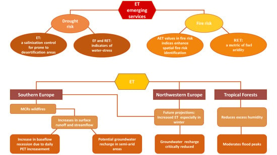
The combined effects which LU/LC change along with climate change triggers on AET should be thoroughly studied since they cause alterations to variables such as albedo, LAI, and root depth which in turn lead to different ET rates [8]. Abatzoglou and Williams (2016) [100] after analyzing the consequences of several fire events in Western continental US forests over 1984–2015, found that anthropogenic climate change is responsible for 2/3 of the increase in RET which, along with VPD, is the most affected parameter by anthropogenic climate change. Therefore, they put forward RET as a metric of fuel aridity, interannually related to the burnt area. Häusler et al. (2019) [101] showed that using AET values acquired by remote sensing in drought indices would enhance the identification of fire risk areas by providing higher resolution. The main interactions between albedo and ET are displayed in Figure 2.
5.2. Post-Fire ET and Groundwater
Poon and Kinoshita (2018) [102] underline the usefulness of evaporation time series, since pre-fire and post-fire biogeological processes would potentially substantially change due to fire disturbances. Alterations in vegetation and soil properties could create a water repellent topsoil layer which would increase surface runoff [102]. Thus, wildfires increase water repellency (or hydrophobicity) of soils, an attribute that substantially affects ET and water infiltration [23]. Johnk and Mays (2021) [103] reported a two-year post-fire reduction of groundwater level in Beaver County, Utah, USA, attributed to the wildfire of 1996. Bart and Tague (2017) [23] examined catchments in California (MCRs), where PET showed a statistically significant impact on baseflow recessions. An increase in the baseflow recession of 33.5% per mm of daily PET increasement has been predicted for eight catchments [23]. Hirano et al. (2015) [99] examined three sites of tropical peat swamp forest in SE Asia. Their results verified that in some settings ET appears strong relationship to groundwater level since the minimum mean value of monthly groundwater level appeared to be a robust predictor of annual ET for peatlands, showing statistically significant positive linearity for all sites despite their different disturbances (i.e., slight drainage, heavy drainage, fire) [99]. Specifically, according to the authors, a drawdown of 10 cm indicates decreases in annual ET between 19–33 mm for the three studied sites [99]. Kurylyk et al. (2015) [104] concluded that the decrease in ET due to canopy loss results in energy excess which warms the land surface. This warming can lead to successive warming of soil water and shallow aquifer water [104], thus ET may indirectly affect groundwater temperature.
These findings are in accordance with the research conducted by Menberg et al. (2014) [105] who underlined the vulnerability of shallow groundwater temperature to disturbances related to climate change.
5.3. Post-Fire ET and Streamflow
Wine and Cadol (2016) [106] suggested that there is a pattern between burn severity magnitude and overland flow in large catchments. Kinoshita and Hogue (2011, 2015) [107,108] found that reduced basin transpiration and infiltration after the wildfire in 2003 in California led to an increase in annual low flow by 118–1090%, which could potentially recharge water supplies in semi-arid areas (Figure 3). On the other hand, elevated flows deliver high loads of sediments. Streamflow increases are reported to sustain for longer than 7 years after the fire depending on the percentage of the burnt area and precipitation, and the types of vegetation loss and reestablishment [107]. Bart (2016) [109] attributed the intense fire effect during the first post-fire year in California to the larger effect on ET which is caused by postfire reductions in shrubland and other vegetation types of the watershed, compared to corresponding post-fire increases in herbaceous vegetation. Since both magnitude and sustainability of post-fire flow depend on scale, Wine and Cadol (2016) [106] highlighted that in large catchments, there is a threshold of 20% affected vegetation of the watershed in order for alterations in hydrogeological processes to have a measurable impact, a finding in line with Bosch and Hewlett’s (1982) [110] research on catchment-scale post-fire ET and water yield.
6. The Anthropogenic Footprint
6.1. Anthropogenic Impacts on ET
The effect of human activities on ET is twofold. One component is atmospheric pollution. The second component is LU/LC change. Global warming has decreased the differences between tropical and polar air temperatures leading to weak global atmospheric circulation, therefore, to a decrease in evaporative demand during past decades [16]. McVicar et al. (2012) [58] suggested that the elevated carbon dioxide concentrations in ambient air during past decades have enhanced vegetation growth. On the other hand, elevated carbon dioxide concentrations lead to a decrease in ET and an increase in soil moisture [111], a finding that may have partially offset the expected increases in ET [77]. Stomatal conductance, which constitutes a direct indicator of plant stress [112], is lower in elevated carbon dioxide environments, thereby decreasing transpiration sometimes by more than 20% [96]. As Liu et al. (2019) [20] demonstrated, an important service of forests is sequestering the carbon of the Earth’s atmosphere. On the other hand, wildfires contribute to carbon dioxide and aerosol accumulation in the atmosphere [20]. However, aerosol is another factor that human activities are primarily accounted for. Wang and Yang (2014) [113] attributed the observed decrease in solar radiation, also referred to as dimming, at North China Plains to aerosols. They also suggested that the decreasing trend in PE in China (evaporation paradox) could be interpreted via surface solar radiation decrease (sunshine hours serve as a proxy of surface solar radiation) [113]. Sun et al. (2018) [9] attributed the decreasing trend in large-pan evaporation during 1985–2008 in North China Plain to the decrease in sunshine hours and VPD. The increasing trend during 2008–2014 was due to the increase in sunshine hours, VPD, and air temperature via heat waves and droughts during summer and spring [9]. Aerosols affect surface energy balance by absorbing and scattering solar radiation. Hallar et al. (2017) [114] refer that organic aerosol increases the optical depth of the atmosphere inhibiting radiation to reach the Earth’s surface. Wildfires constitute significant sources of organic aerosols and are projected to increase optical depth in West US during summertime by 40% until 2050 [114]. As a result, net radiation is reduced by aerosol accumulation from anthropogenic emissions [17]. Jiang et al. (2019) [16] interpreted the larger magnitude of increase in minimum air temperature compared to maximum air temperature (also reported in Central Italy [115]) by the action of aerosols which absorb a part of solar radiation and emit longwave radiation at night. Industrialization of the recent decades in several regions in East Asia led to a significant increase in aerosol aggregation. However, in contradiction to East Asia, Central Mediterranean and NE America exhibited downward trends of aerosol optical depth in the 2000s as a result of the enforcement of emission-decreasing policies [116]. Urbanization density has been correlated with aerosol accumulation by Zhao et al. (2014) [117] in China, while it is asserted that high buildings in big cities inhibit aerosol diffuse by blocking wind flow, thus contributing to a decrease in solar radiation [17].
Human activities such as LU/LC change over the past decades account for ET variations by several researchers. Lv et al. (2019) [8] analyzed AET between 1986–2016 in the Yellow River basin. They found that the extended LU/LC change including conversion of the sloped terrain into terraced fields, dam constructions, forest, and vegetation implementation led to an increase in AET. They concluded that 90% of the AET increase was due to human activities and only 10% due to precipitation shift [8]. They attributed the former ratio for the thirty-year period to the reduction in surface runoff and to the increase in vegetation which increased the AET. The LU/LC changes affect the values of the physical parameter called “surface roughness”. Human activities often increase the surface roughness. Even McVicar et al. (2012) [58] asserted that vegetation cover was due to agricultural abandonment of lands, surface roughness was shown to be increased due to agricultural land expansion [16]. The latter can be explained by the intensification of crop yielding the years following the former study, especially across specific areas (e.g., California). For example, Mueller et al. (2017) [77] referred that cropland expansion could affect climate by changing, among other parameters, the surface roughness. It seems that vegetation greenness along with agricultural land expansion affect AET variations by increasing surface roughness [8]. McVicar et al. (2012) [58], after analyzing numerous studies, concluded that terrestrial (wind) stilling has been observed in many regions globally during the last 30 years and led to a decline in evaporative demand reflected on PE and RET measurements.
6.2. Agricultural Practices Affect ET
The impacts of agricultural plantations on ET variations have attracted the interest of researchers especially at regions with high rates of crop yield and financial interest. Mueller et al. (2017) asserted that intensification of productivity, which incorporates extended irrigation, influences climate via increasing ET [77]. This fact results in regional cooling effect in accordance with the globally documented cooling trend in intensified croplands over the last decades, compared to adjacent regions. This could be attributed to the mediating role of vegetation in land–atmosphere coupling through controlling surface energy fluxes such as ET [118]. Irrigation directly affects the hydrological cycle of an area and the extra water on the soil enhances AET rates [1,119]. Uddin et al. (2016) studied the case of a cotton crop in Queensland, Australia (subtropical climate), during irrigation events, concluding that irrigation also changes the albedo value of the (wet) canopy [5]. They found that both during and following an irrigation event a considerable amount of the intercepted water evaporates: 11% of the applied water evaporates in highly advective conditions, while 8% in non-advective conditions [5]. Irrigation of croplands has been reported to increase ET in several regions globally such as the U.S., Asia, and Sudan [77]. The implementation of specific practices, such as multi-cropping, enhanced seasonal variation of ET at Brazilian Cerrado and North China Plain [77]. In addition, the availability of nitrogen at croplands (e.g., via land application of fertilizers, amendments, and biosolids [120]) has been correlated with an increase in ET since nitrogen availability is a limiting factor that governs plant biochemical processes (stomatal conductance, water uptake, photosynthesis) [121]. García-Llamas et al. (2019) underlined that PET is associated with the theoretical limit of the process of photosynthesis of plants [122]. French et al. (2016) asserted that a measure of relative ET such as the evaporative fraction (EF), which is a key factor in energy balance algorithms (equal to the ratio of latent heat flux to available land surface energy; [123]) could serve as a water stress indicator [124].
Irrigation decision making relies on the accuracy of ET estimations which in cases of remote sensing approaches depends on the overpass frequencies. Remote sensing is the usual approach for district-scale (regional) estimation, often used for fields too (local scale). French et al. (2016) [124] found significant benefit in ET accuracy when 8-day satellite ET products were used instead of 16-day products. The differences of seasonal water use estimation between 8-day and 16-day overpassing were up to 20%, suggesting considerable implications in regional water management in the second case.
6.3. ET Potentially Aggravates Soil Water and Groundwater Pollution
Nitrogen stress constitutes a control on ET rates by hindering the stomatal conductance, the leaf area, and the root development [77]. Post-fire ash is enriched in nutrients but is easily erodible and transported by wind and foremost by runoff. After intense rainfall events, nutrients are eluted from the topsoil layer. Recurrences of fires over the same site deteriorate soil deprivation in nutrients [125], jeopardizing stream water quality and, potentially, shallow aquifer or karst aquifer water quality which are vulnerable to pollution [126,127]. Tsypkin and Brevdo (1999) [128] after studying the evaporation impacts on groundwater quality, indicated a mechanism of pollutant deposition in groundwater caused by ET. They found that evaporation produces a gradient of the solute concentration with a vertical upward direction. For certain substances, such as NaCl, the maximum concentration at the evaporation front was greater than solubility, the latter defined as the critical concentration above which pollutant deposition begins [128]. Gran et al. (2009) [129] explained that the evaporation front divides soil into the upper dry area with salt content and the one below the front where salinity is low, suggesting that evaporation could serve as a moderating control on soil salinization since at least half of irrigated lands in arid and semi-arid regimes are subject to some degree of salinization). The salinization of soil has been correlated to erosion and desertification [130] and also to the salinization of rainfall that reaches the soil [131]. Considerable salt load is transported to freshwater ecosystems via runoff with potential salinization risk for shallow aquifers [131]. This conclusion becomes of major importance in the ongoing climate crisis. Chen et al. (2015) [132] reported that there has been a global increase in drought land since the late 1990s, with those in humid areas being the most concerning. They found that the ongoing air temperature rise accounts for 5% (humid areas) up to 45% (arid areas) of droughts in China [132]. On the other hand, high ET rates inhibit the infiltration of dissolved pollutants towards the aquifers. The evaporation enrichment concerns croplands’ irrigation applied during periods when the evaporative demand is high, hence salt enrichment is considerable [133]. This water enriched in salts could potentially reach the aquifer triggering a cycle of successive enrichment if the enriched groundwater is pumped and used for irrigation, depending on the depth of the unsaturated zone, water fluxes in the saturated zone, and the evaporation rate [133]. The former process could lead to enhanced enrichment in cases where reclaimed water with high salt content is used for irrigation [134], a practice that has gained popularity not only for croplands but also for forests [135,136].
7. Discussion
This review has been carried out following the appropriate steps of a structured review [52,53,137] as shown in Figure 1, analyzing 141 studies, the majority of which were published during the last decade. The main findings are presented below:
ET is beneficial to tropical forests since it reduces excess humidity, moderating flood peaks [93] (see Figure 3). Moreover, ET could serve as a salinization control for regions endangered by desertification (see Figure 2).
A decrease in AET was found to be responsible for post-fire warming at a global scale after the extended wildfires during 2003–2014 [20]. The latter resulted in an increase in albedo which consequently reduced the net cooling effect [20]. The cooling effect is typical across tropical forests due to the high AET rates. However, the vegetation loss in tropical forests reduced the evaporative cooling resulting in a rise in the air temperature [20].
Moreover, droughts often increase albedo whereas studded open water after wildfires results in decreased albedo [99]. Overall, interactions between ET and albedo in different ecosystems govern surface warming and radiation budget responses [20] (see Figure 2). LE contributions of soil and canopy can be almost interchanged shortly after the fire [95].
Fire severity has been associated with AET differences in MCRs (see Figure 3) and with the number of years needed for AET to rebound to pre-fire levels [95,96,97].
ET rates affect groundwater recharge (see Figure 3). Projections for years 2071–2100 in Italy showed an increase in ET by 25% in winter, at least by 20% in fall, and by 15% in summer. This projection along with the anticipated alterations in precipitation patterns led to predicted groundwater recharge critically reduced in South Mediterranean [88]. However, this is not the case only for the endangered of high warming and drought in Southern Europe [60,138], which as a rule exhibits different precipitation patterns to North Europe. According to projections of ET for 2020 and 2080 in Ireland, North Europe is also anticipated to be critically affected [2]. Canopy removal reduces transpiration and can lead to increases in low baseflow and streamflow by 118–1090%. These alterations can sustain more than 7 years as reported in California (MCRs) [107,108]. This fact could be beneficial for groundwater recharge in semi-arid areas. The sustaining increases in low flow were also linked to the severity of the fire. Researchers concluded that 20% canopy removal from a catchment could be considered as a threshold above which alterations in hydrological processes occur [106,110]. Across MCRs, PET appeared statistically significant impact on baseflow recessions, quantified as a 33.5% increase in baseflow recession per 1 mm of daily PET increasement [23]. Furthermore, the minimum mean value of monthly groundwater level appeared to be a predictor of annual ET across tropical peat swamp forests in SE Asia, despite the different regional disturbances (see Figure 3). This relationship appears linearity: drawdown of 10 cm led to a decrease in annual ET by 19–33 mm [99].
Anthropogenic climate change has been accounted for 2/3 of the increase in RET [94]. The latter, along with VPD, appeared to be the most affected meteorological parameters, thus Abatzoglou and Williams (2016) [100] put forward RET as a metric of fuel aridity. It has been also shown by Häusler et al. (2019) [101] that AET values in fire risk indices would enhance spatial fire risk identification. Moreover, RET estimates constitute an indicator of water stress in areas prone to drought [139].
Wind stilling is the phenomenon responsible for the majority of decreasing ET trends during past decades on a global scale [58]. Wind stilling has been associated with the observed increase in surface roughness and led to a decrease in evaporative demand and successively to a decline of PE and RET values during past decades [8,58] (see Figure S1 on evaporation paradox in Supplementary Materials). According to McVicar et al. (2012) [58], the aforementioned drivers could explain the Evaporation paradox reported in several countries of the globe (see Figure S1 in Supplementary Materials). Roderick and Farquhar (2004) [85] shared the same opinion. However, in numerous countries, a rebound of PE occurred during the decades of 1980 and 1990. According to ET trends, benchmarks of ET rebound have been reported in the early to middle 1980s for Greece [64], Iran [1], and Nigeria [66], and in the 1990s for China [16,20] and Australia [87], while South Florida also exhibited an increasing trend at least since 1992 [79]. Air pollution is likely to affect ET rates: elevated carbon dioxide concentrations in the ambient air can decrease transpiration in some cases by more than 20% [77]. The latter may have offset the anticipated increase in ET trends [77]. Another phenomenon that has been accounted for decreasing trends in ET is global dimming, attributed to aerosol accumulation over past decades linked to industrialization and urbanization (see Figure S1). Global dimming was followed by global brightening [65,140,141]. The observed increase in solar and thermal radiative heating after the mid-1980s facilitated the intensification of the hydrological cycle and scattered aerosol loads [140,141]. For instance, the delay of ET rebound in China compared to Greece as reported above [9,64], is in line with the findings by Zerefos et al. (2009) [142] regarding the periods when the rebound in aerosol optical depth (brightening) was observed in those countries.
Several researchers have examined ET variations in light of the anthropogenic footprint. Lv et al. (2019) [8] deducted that 90% of the reported increase in AET was due to human activities and only 10% due to shifted and altered precipitation patterns which are associated with the climate crisis. AET was increased as a result of LU/LC shift towards large constructions such as dams, vegetation implementation (e.g., agriculture), and implemented reforestation. In addition, intensification of agricultural productivity involving extended irrigation and no-till and fallow practices increased ET via albedo, resulting in some cases (e.g., USA) in regional net cooling effect [8,77] (see Figure 2). Nitrogen availability has been also associated with elevated transpiration rates since nutrients constitute a limiting factor for plants’ biophysiological processes. Nutrient sources are chemical fertilizers, amendments, raw sludge, or biosolids from wastewater treatment plants, and wastewater overflows which end up in natural receivers. In addition, some amount of nutrients also becomes available by the usage of fire retardants during fire distinguishing, since their composition resembles that of fertilizers [126,127] (see Figure 2).
It is apparent that the anthropogenic footprint in LU/LC, ambient air, and climate change have affected ET rates globally. Even if the evaporation paradox can be approached, the changeable climate patterns along with the significance of ET impacts on ecosystems, water supplies, and sustainability call for systematic research on PET, RET, PE, and AET to many more countries with different environmental conditions, aiming to quantify the relations between them [46,87,143]. Moreover, the mechanisms in which ET participates are related to cropland irrigation and practices, forest implementation, LU/LC management, fire management (preventing and mitigating), and water management (surface waterbodies and aquifers). Thus, it is recommended that stakeholders (scientists, engineers, water managers, and policymakers) consider the integrated role of ET in the elaborated mechanisms.
8. Conclusions
Climate change along with LU/LC change have aggravated or even triggered alterations to climatic variables and disturbances such as frequent droughts and extended wildfires which enlarge the effects of ET in the hydrological cycle and the surface energy balance. Thus, ET constitutes a major control of the prementioned processes. The specific hydrogeological, physical, and topographical characteristics along with the dynamics of regional climate conditions in the frame of the ongoing climate change practically turn each study area into a case study. Complex interactions and dynamics of several combinations of meteorological, lithological, hydrogeological, and physiological components with ET cannot lead to the formation of a general pattern of ET behavior or be reproduced, due to the nature of those relationships and the fact that numerous interfering factors such as weather conditions appearing temporal variability or even stochasticity govern the outcomes of the hydrological processes. Moreover, the review has a qualitative character and the deducted conclusions cannot be quantified. Consequently, the limitations of the present study are the impracticability of quantification and broad generalization. The latter could result in overgeneralization and oversimplification of mechanisms and interactions with many degrees of freedom. Furthermore, although all the main climate zones are covered, the review focuses on areas with considerable water-stress and desertification issues as the latter constitute severe impacts of climate change, bearing socio-economic consequences.
However, in some climate zones, some common behaviors of hydrological interactions could be detected, still need thorough future investigation aiming patterns to be extracted. This study does not aspire to discuss all possible interactions and impacts of ET in the environment. Instead, this study aims at setting the foundation for future research which addresses the integrated picture of ET as a major controlling factor of climate and sustainability. It provides a general overview of the main mechanisms in which ET participates, by pointing out the main interactions between ET, key environmental variables, and disturbances in different settings. Overall, since useful literature-based connections were made for specific areas under specific environmental conditions the former limitations are not considered critical for the validity of the conclusions.
Five broad conclusions can be deducted: First, MCRs appear to be vulnerable to the impacts of the ongoing increase in ET, especially during summertime, due to the ongoing precipitation shifting in winter and the air temperature warming (especially the rise of minimum air temperature values) which is expected to be more severe in MCRs such as Southern Europe, in the summertime. Air temperature is considered as a proxy of the energy state of the system. In water-limited areas, EF could serve as a water-stress indicator. Second, ET in tropical forests plays a rather beneficial role since it moderates the flooding risk during the wet season resulting in a net cooling effect. Third, in semi-arid to arid areas, an increase in ET and especially of evaporation constitutes an important problem due to sustained baseflow recessions which aggravate the limited water availability. In those drought-prone areas, ET exacerbates soil salinization. Fourth, the relationship between ET and wildfires is of major importance. The impacts are site-specific, climate, and fire-severity-dependent. The hydrological processes may be altered if a critical amount of canopy loss (e.g., 20% for semi-arid regions, 45% for tropical forests) occurs. Concurrently, RET could serve as a fuel aridity measure to assess forest fire risk. The case of Australia, with high rates of evaporation reported, may be a verification of the former deduction. Fifth, along with climate change, human activity consequences such as air pollution (aerosols, CO2 emissions), LU/LC shifting to agricultural uses with intensive productivity practices, large reforestation implementation, and large constructions (e.g., dams, dense and high urban buildings) have substantially changed AET rates during last decades. Via the human footprint, the interpretation of the evaporation paradox has been made plausible.
In this context, future research is proposed to be designed towards two complementary axons. First, more refined, sophisticated ET modeling for global, regional, and local scales employing remote sensing techniques can be supported by eddy covariance, lysimeter, or pan evaporation measurements. Second, investigations that assess and quantify the dynamic anthropogenic impact on ET variability, aiming scientists, engineers as well as water managers to consider ET as a means to address the challenging environmental issues in two axons; either by finding methods to control it or by using it as an index of fire risk or water stress to help prevent or mediate the climate change impacts on water availability.
Supplementary Materials
The figure showing the evaporation paradox is available online at https://www.mdpi.com/article/10.3390/hydrology8040163/s1, Figure S1: Anthropogenic derived concepts which contribute to the interpretation of the evaporation paradox.
Author Contributions
Conceptualization, S.D. and K.G.N.; methodology, S.D. and K.G.N.; investigation, S.D.; data curation, S.D.; writing—original draft preparation, S.D.; writing—review and editing, S.D. and K.G.N.; supervision, K.G.N. All authors have read and agreed to the published version of the manuscript.
Funding
This research received no external funding.
Institutional Review Board Statement
Not applicable.
Informed Consent Statement
Not applicable.
Acknowledgments
Authors acknowledge the two anonymous reviewers for their contribution.
Conflicts of Interest
Authors declare no conflict of interest.
References
- Xu, S.; Yu, Z.; Yang, C.; Ji, X.; Zhang, K. Trends in evapotranspiration and their responses to climate change and vegetation greening over the upper reaches of the Yellow River Basin. Agric. For. Meteorol. 2018, 263, 118–129. [Google Scholar] [CrossRef]
- Gharbia, S.S.; Smullen, T.; Gill, L.; Johnston, P.; Pilla, F. Spatially distributed potential evapotranspiration modeling and climate projections. Sci. Total Environ. 2018, 633, 571–592. [Google Scholar] [CrossRef] [PubMed]
- Ampas, V.; Baltas, E. Sensitivity analysis of different evapotranspiration methods using a new sensitivity coefficient. Glob NEST J. 2012, 14, 335–343. Available online: https://journal.gnest.org/sites/default/files/Journal%20Papers/335-343_882_Ambas_14_3.pdf (accessed on 29 October 2021).
- Bulcock, H.H.; Jewitt, G.P.W. Modelling canopy and litter interception in commercial forest plantations in South Africa using the Variable Storage Gash model and idealised drying curves. Hydrol. Earth Syst. Sci. 2012, 16, 4693–4705. [Google Scholar] [CrossRef] [Green Version]
- Uddin, J.; Foley, J.P.; Smith, R.J.; Hancock, N.H. A new approach to estimate canopy evaporation and canopy interception capacity from evapotranspiration and sap flow measurements during and following wetting. Hydrol. Process. 2016, 30, 1757–1767. [Google Scholar] [CrossRef]
- Tegos, A.; Efstratiadis, A.; Koutsoyiannis, D. A Parametric Model for Potential Evapotranspiration Estimation Based on a Simplified Formulation of the Penman-Monteith Equation, Evapotranspiration—An Overview; Alexandris, S.G., Ed.; InTech: Rijeka, Croatia, 2013; Available online: https://www.intechopen.com/chapters/44363 (accessed on 29 October 2021). [CrossRef] [Green Version]
- Yang, Y.; Chen, R.; Song, Y.; Han, C.; Liu, J.; Liu, Z. Sensitivity of potential evapotranspiration to meteorological factors and their elevational gradients in the Qilian Mountains, northwestern China. J. Hydrol. 2019, 568, 147–159. [Google Scholar] [CrossRef]
- Lv, X.; Zuo, Z.; Sun, J.; Ni, Y.; Wang, Z. Climatic and human-related indicators and their implications for evapotranspiration management in a watershed of Loess Plateau, China. Ecol. Indic. 2019, 101, 143–149. [Google Scholar] [CrossRef]
- Sun, Z.; Ouyang, Z.; Zhao, J.; Li, S.; Zhang, X.; Ren, W. Recent rebound in observational large-pan evaporation driven by heat wave and droughts by the Lower Yellow River. J. Hydrol. 2018, 565, 237–247. [Google Scholar] [CrossRef]
- Allen, R.; Pereira, L.; Raes, D.; Smith, M. Crop evapotranspiration–Guidelines for computing crop water requirements. In Irrigation and Drainage; Paper No. 56; FAO: Rome, Italy, 1998; Volume 300. [Google Scholar]
- Fu, G.; Liu, C.; Chen, S.; Hong, J. Investigating the conversion coefficients for free water surface evaporation of different evaporation pans. Hydrol. Process. 2014, 18, 2247–2262. [Google Scholar] [CrossRef]
- Masoner, J.R.; Stannard, D.I.; Christenson, S.C. Differences in Evaporation Between a Floating Pan and Class A Pan on Land. J. Am. Water Resour. Assoc. 2018, 44, 552–561. [Google Scholar] [CrossRef]
- Kitsara, G.; Papaioannou, G.; Retalis, A.; Paronis, D.; Kerkides, P. Estimation of air temperature and reference evapotranspiration using MODIS land surface temperature over Greece evapotranspiration using MODIS land surface temperature. Int. J. Remote Sens. 2018, 39, 924–948. [Google Scholar] [CrossRef]
- Zamani Losgedaragh, S.; Rahimzadegan, M. Evaluation of SEBS, SEBAL, and METRIC models in estimation of the evaporation from the freshwater lakes (Case study: Amirkabir dam, Iran). J. Hydrol. 2018, 561, 523–531. [Google Scholar] [CrossRef]
- Kim, S.; Kim, H.S. Neural networks and genetic algorithm approach for nonlinear evaporation and evapotranspiration modeling. J. Hydrol. 2008, 351, 299–317. [Google Scholar] [CrossRef]
- Jiang, S.; Liang, C.; Cui, N.; Zhao, L.; Du, T.; Hu, X.; Feng, Y.; Guan, J.; Feng, Y. Impacts of climatic variables on reference evapotranspiration during growing season in Southwest China. Agric. Water Manag. 2019, 216, 365–378. [Google Scholar] [CrossRef]
- Fan, J.; Wu, L.; Zhang, F.; Xiang, Y.; Zheng, J. Climate change effects on reference crop evapotranspiration across different climatic zones of China during 1956–2015. J. Hydrol. 2016, 542, 923–937. [Google Scholar] [CrossRef]
- McCuen, H.R. A sensitivity and error analysis of procedures used for estimating evapotranspiration. Water Resour. Bull. 1974, 10, 486–498. [Google Scholar] [CrossRef]
- Wang, Z.; Xie, P.; Lai, C.; Chen, X.; Wu, X.; Zeng, Z.; Li, J. Spatiotemporal variability of reference evapotranspiration and contributing climatic factors in China during 1961–2013. J. Hydrol. 2017, 544, 97–108. [Google Scholar] [CrossRef]
- Liu, Z.; Ballantyne, A.P.; Cooper, L.A. Biophysical feedback of global forest fires on surface temperature. Nat. Commun. 2019, 10, 1–9. [Google Scholar] [CrossRef] [Green Version]
- Tie, Q.; Hu, H.; Tian, F.; Holbrook, N.M. Comparing different methods for determining forest evapotranspiration and its components at multiple temporal scales. Sci. Total Environ. 2018, 633, 12–29. [Google Scholar] [CrossRef]
- Xiao, Q.; McPherson, E.; Ustin, L.; Grismer, M.; Simpson, J. Winter rainfall interception by two mature open-grown trees in Davis, California. Hydrol. Process. 2000, 14, 763–784. [Google Scholar] [CrossRef]
- Bart, R.R.; Tague, C.L. The impact of wildfire on baseflow recession rates in California. Hydrol. Process. 2017, 31, 1662–1673. [Google Scholar] [CrossRef]
- Guevara-Escobar, A.; Gonzalez-Sosa, E.; Veliz-Chavez, C.; Ventura-Ramos, E.; Ramos-Salinas, M. Rainfall interception and distribution patterns of gross precipitation around an isolated Ficus benjamina tree in an urban area. J. Hydrol. 2007, 333, 532–541. [Google Scholar] [CrossRef]
- Williams, D.G.; Cable, W.; Hultine, K.; Hoedjes, J.C.B.; Yepez, E.A.; Simonneaux, V.; Er-Raki, S.; Boulet, G.; de Bruin, H.A.R.; Chehbouni, A.; et al. Evapotranspiration components determined by stable isotope, sap flow and eddy covariance techniques. Agric. For. Meteorol. 2004, 125, 241–258. [Google Scholar] [CrossRef]
- Qiu, X.; Zhang, M.; Wang, S.; Argiriou, A.A.; Chen, R.; Meng, H.; Guo, R. Water Stable Isotopes in an Alpine Setting of the Northeastern Tibetan Plateau. Water 2019, 11, 770. [Google Scholar] [CrossRef] [Green Version]
- Shi, M.; Wang, S.; Argiriou, A.A.; Zhang, M.; Guo, R.; Jiao, R.; Kong, J.; Zhang, Y.; Qiu, X.; Zhou, S. Stable Isotope Composition in Surface Water in the Upper Yellow River in Northwest China. Water 2019, 11, 967. [Google Scholar] [CrossRef] [Green Version]
- Gokmen, M.; Vekerdy, Z.; Verhoef, A.; Verhoef, W.; Batelaan, O.; van der Tol, C. Integration of soil moisture in SEBS for improving evapotranspiration estimation under water stress conditions. Remote Sens. Environ. 2012, 121, 261–274. [Google Scholar] [CrossRef]
- Valipour, M.; Gholami Sefidkouhi, M.A.; Raeini−Sarjaz, M. Selecting the best model to estimate potential evapotranspiration with respect to climate change and magnitudes of extreme events. Agric. Water Manag. 2017, 180, 50–60. [Google Scholar] [CrossRef]
- Mu, Q.; Zhao, M.; Running, S.W. Improvements to a MODIS global terrestrial evapotranspiration algorithm. Remote Sens. Environ. 2011, 115, 1781–1800. [Google Scholar] [CrossRef]
- Allen, R.G.; Tasumi, M.; Morse, A.; Trezza, R. A Landsat-based energy balance and evapotranspiration model in Western US water rights regulation and planning. Irrig Drain. Syst. 2005, 19, 251–268. [Google Scholar] [CrossRef]
- Anderson, M.C.; Kustas, W.P.; Norman, J.M.; Hain, C.R.; Mecikalski, J.R.; Schultz, L.; González-Dugo, M.P.; Cammalleri, C.; d’Urso, G.; Pimstein, A.; et al. Mapping daily evapotranspiration at field to continental scales using geostationary and polar orbiting satellite imagery. Hydrol. Earth Syst. Sci. 2015, 15, 223–239. [Google Scholar] [CrossRef] [Green Version]
- Bastiaanssen, W.G.M.; Menenti, M.; Feddes, R.A.; Holtslag, A.A.M. A remote sensing surface energy balance algorithm for land (SEBAL). 1. Formulation. J. Hydrol. 1998, 212–213, 198–212. [Google Scholar] [CrossRef]
- Sánchez, J.M.; Kustas, W.P.; Caselles, V.; Anderson, M.C. Modelling surface energy fluxes over maize using a two-source patch model and radiometric soil and canopy temperature observations. Remote Sens. Environ. 2008, 112, 1130–1143. [Google Scholar] [CrossRef]
- Su, B.; Wang, L. Earth Observation of Water Resources (SEBS), Teaching Presentation, University of Twente The Netherlands. 2013. Available online: https://earth.esa.int/documents/10174/643007/D5P1c-1_SEBS_LTC2013.pdf (accessed on 9 September 2021).
- Dimitriadou, S.; Nikolakopoulos, K.G. Remote sensing methods to estimate evapotranspiration incorporating MODIS derived data and applications over Greece: A review. In Proceedings of the SPIE 11524, Eighth International Conference on Remote Sensing and Geoinformation of the Environment (RSCy2020), Paphos, Cyprus, 26 August 2020. [Google Scholar]
- Tabari, H.; Grismer, M.E.; Trajkovic, S. Comparative analysis of 31 reference evapotranspiration methods under humid conditions. Irrig. Sci. 2013, 31, 107–117. [Google Scholar] [CrossRef]
- Malamos, N.; Tsirogiannis, I.L.; Tegos, A.; Efstratiadis, A.; Koutsoyiannis, D. Spatial interpolation of potential evapotranspiration for precision irrigation purposes. Eur. Water 2017, 59, 303–309. Available online: https://www.itia.ntua.gr/el/getfile/1776/1/documents/EW_2017_59_41_2HOxTxv.pdf (accessed on 9 September 2021).
- Vasiliades, L.; Spiliotopoulos, M.; Tzabiras, J.; Loukas, A.; Mylopoulos, N. Estimation of crop water requirements using remote sensing for operational water resources management. In Proceedings of the Third International Conference on Remote Sensing and Geoinformation of the Environment (RSCy2015) SPIE 9535, Paphos, Cyprus, 19 June 2015; p. 95351B. [Google Scholar]
- Demertzi, K.; Pisinaras, V.; Lekakis, E.; Tziritis, E.; Babakos, K.; Aschonitis, V. Assessing Annual Actual Evapotranspiration based on Climate, Topography and Soil in Natural and Agricultural Ecosystems. Climate 2021, 9, 20. [Google Scholar] [CrossRef]
- Dimitriadou, S.; Nikolakopoulos, K.G. Annual Actual Evapotranspiration Estimation via GIS Models of Three Empirical Methods Employing Remotely Sensed Data for the Peloponnese, Greece, and Comparison with Annual MODIS ET and Pan Evaporation Measurements. ISPRS Int. J. Geo-Inf. 2021, 10, 522. [Google Scholar] [CrossRef]
- Dimitriadou, S.; Nikolakopoulos, K.G. Reference evapotranspiration (ETo) methods implemented as ArcMap models with remote sensed and ground-based inputs, examined along with MODIS ET, for Peloponnese, Greece. ISPRS Int. J. Geo-Inf. 2021, 10, 390. [Google Scholar] [CrossRef]
- Anderson, E. Calibration of Conceptual Hydrologic Models for Use in River Forecasting. NOAA Technical Report, NWS 45, Hydrology Laboratory, August 2002. Available online: https://www.semanticscholar.org/paper/Calibration-of-Conceptual-Hydrologic-Models-for-Use-Anderson/9ec4749a4064e6d41058c8c6fbcda108210e6865#paper-header (accessed on 10 September 2021).
- Herman, M.R.; Nejadhashemi, A.P.; Abouali, M.; Hernandez-Suarez, J.S.; Daneshvar, F.; Zhang, Z.; Anderson, M.C.; Sadeghi, A.M.; Hain, C.R.; Sharifi, A. Evaluating the role of evapotranspiration remote sensing data in improving hydrological modeling predictability. J. Hydrol. 2018, 556, 39–49. [Google Scholar] [CrossRef]
- Zhao, T.; Wang, Q.J.; Schepen, A.; Griffiths, M. Ensemble forecasting of monthly and seasonal reference crop evapotranspiration based on global climate model outputs. Agric. For. Meteorol. 2019, 264, 114–124. [Google Scholar] [CrossRef]
- Johnson, F.; Sharma, A. A Comparison of Australian Open Water Body Evaporation Trends for Current and Future Climates Estimated from Class A Evaporation Pans and General Circulation Models. J. Hydrometeor. 2010, 11, 105–121. [Google Scholar] [CrossRef]
- Sattari, M.T.; Apaydin, H.; Band, S.S.; Mosavi, A.; Prasad, R. Comparative analysis of kernel-based versus ANN and deep learning methods in monthly reference evapotranspiration estimation. Hydrol. Earth Syst. Sci. 2021, 25, 603–618. [Google Scholar] [CrossRef]
- Tegos, A.; Efstratiadis, A.; Malamos, N.; Mamassis, N.; Koutsoyiannis, D. Evaluation of a Parametric Approach for Estimating Potential Evapotranspiration Across Different Climates. Agric. Agric. Sci. Procedia 2015, 4, 2–9. [Google Scholar] [CrossRef] [Green Version]
- Batra, K.; Gandhi, P. Neural Network-Based Prediction Model for Evaporation Using Weather Data. Agric. Res. 2021. [Google Scholar] [CrossRef]
- Malik, A.; Kumar, A.; Kisi, O. Monthly pan-evaporation estimation in Indian central Himalayas using different heuristic approaches and climate based models. Comput. Electron. Agric. 2017, 143, 302–313. [Google Scholar] [CrossRef]
- Güçlü, Y.S.; Subyani, A.M.; Şen, Z. Regional fuzzy chain model for evapotranspiration estimation. J. Hydrol. 2017, 544, 233–241. [Google Scholar] [CrossRef]
- Boaz, A.; Ashby, D.; Young, K. Systematic Reviews: What Have They Got to Offer Evidence Based Policy and Practice? ESRC UK Centre for Evidence Based Policy and Practice, Queen Mary University of London, UK, 1–26. Available online: https://emilkirkegaard.dk/en/wp-content/uploads/Should-I-do-a-systematic-review.pdf (accessed on 10 September 2021).
- Gill, J.C.; Malamud, B.D. Anthropogenic processes, natural hazards, and interactions in a multi-hazard framework. Earth-Sci. Rev. 2017, 166, 246–269. [Google Scholar] [CrossRef] [Green Version]
- Hobbins, M.T.; Ramirez, J.A.; Brown, T.C. Trends in pan evaporation and actual evapotranspiration across the conterminous U.S.: Paradoxical or complementary? Geophys. Res. Lett. 2004, 31, 1–5. [Google Scholar] [CrossRef] [Green Version]
- Qin, M.; Zhang, Y.; Wan, S.; Yue, Y.; Cheng, Y.; Zhang, B. Impact of climate change on “evaporation paradox” in province of Jiangsu in southeastern China. PLoS ONE 2021, 16, e0247278. [Google Scholar] [CrossRef]
- Ohmura, A.; Wild, M. Is the hydrological cycle accelerating? Science 2002, 298, 1345–1346. [Google Scholar] [CrossRef]
- Burn, D.H.; Hesch, N.M. Trends in evaporation for the Canadian Prairies. J. Hydrol. 2007, 336, 61–73. [Google Scholar] [CrossRef]
- McVicar, T.R.; Roderick, M.L.; Donohue, R.J.; Li, L.T.; Van Niel, T.G.; Thomas, A.; Grieser, J.; Jhajharia, D.; Himri, Y.; Mahowald, N.M.; et al. Global review and synthesis of trends in observed terrestrial near-surface wind speeds: Implications for evaporation. J. Hydrol. 2012, 416, 182–205. [Google Scholar] [CrossRef]
- Wang, M.; Zhang, Y.; Lu, Y.; Gong, X.; Gao, L. Detection and attribution of reference evapotranspiration change (1951–2020) in the Upper Yangtze River Basin of China. J. Water Clim. Chang. 2021, 12, 2624–2638. [Google Scholar] [CrossRef]
- You, G.; Zhang, Y.; Liu, Y.; Song, Q.; Lu, Z.; Tan, Z.; Wu, C.; Xie, Y. On the attribution of changing pan evaporation in a nature reserve in SW China. Hydrol. Process. 2013, 27, 2676–2682. [Google Scholar] [CrossRef]
- Liu, X.; Luo, Y.; Zhang, D.; Zhang, M.; Liu, C. Recent changes in pan-evaporation dynamics in China. Geophys. Res. Lett. 2011, 38, L13404. [Google Scholar] [CrossRef] [Green Version]
- Jhajharia, D.; Shrivastava, S.K.; Sarkar, D.; Sarkar, S. Temporal characteristics of pan evaporation trends under the humid conditions of northeast India. Agric. For. Meteorol. 2009, 149, 763–770. [Google Scholar] [CrossRef]
- Maček, U.; Bezak, N.; Šraj, M. Reference evapotranspiration changes in Slovenia, Europe. Agric. For. Meteorol. 2018, 260, 183–192. [Google Scholar] [CrossRef]
- Papaioannou, G.; Kitsara, G.; Athanasatos, S. Impact of global dimming and brightening on reference evapotranspiration in Greece. J. Geophys. Res. 2011, 116, D09107. [Google Scholar] [CrossRef]
- Kitsara, G.; Papaioannou, G.; Papathanasiou, A.; Retalis, A. Dimming/brightening in Athens: Trends in Sunshine Duration, Cloud Cover and Reference Evapotranspiration. Water Resour. Manag. 2013, 27, 1623–1633. [Google Scholar] [CrossRef]
- Ogolo, E.O. Regional trend analysis of pan evaporation in Nigeria (1970 to 2000). J. Geogr. Reg. Plan. 2011, 4, 566–577. Available online: https://pdfs.semanticscholar.org/57a9/ce191a35968d7e6ab147416b24ce3e64f852.pdf (accessed on 8 September 2021).
- Cohen, S.; Ianetz, A.; Stanhill, G. Evaporative climate changes at Bet Dagan, Israel, 1964–1998. Agric. For. Meteorol. 2002, 111, 83–91. [Google Scholar] [CrossRef]
- Dadaser-Celik, F.; Cengiz, E.; Guzel, O. Trends in reference evapotranspiration in Turkey: 1975–2006. Int. J. Climatol. 2016, 36, 1733–1743. [Google Scholar] [CrossRef] [Green Version]
- Yeşilırmak, E. Temporal changes of warm-season pan evaporation in a semi-arid basin in Western Turkey. Stoch Environ. Res. Risk Assess. 2013, 27, 311–321. [Google Scholar] [CrossRef]
- Lionello, P.; Scarascia, L. The relation between climate change in the Mediterranean region and global warming. Reg. Environ. Chang. 2018, 18, 1481–1493. [Google Scholar] [CrossRef]
- Vicente-Serrano, S.M.; Bidegain, M.; Tomas-Burguera, M.; Dominguez-Castro, F.; El Kenawy, A.; McVicar, T.R.; Azorin-Molina, C.; López-Moreno, J.I.; Nieto, R.; Gimeno, L.; et al. A comparison of temporal variability of observed and model-based pan evaporation over Uruguay (1973–2014). Int. J. Climatol. 2018, 38, 337–350. [Google Scholar] [CrossRef]
- Breña-Naranjo, J.A.; Laverde-Barajas, M.Á.; Pedrozo-Acuña, A. Changes in pan evaporation in Mexico from 1961 to 2010. Int. J. Climatol. 2017, 37, 204–213. [Google Scholar] [CrossRef]
- Aschonitis, V.; Miliaresis, G.; Demertzi, K.; Papamichail, D. Terrain Segmentation of Greece Using the Spatial and Seasonal Variation of Reference Crop Evapotranspiration. Adv. Meteorol. 2016, 1–14. [Google Scholar] [CrossRef] [Green Version]
- Estévez, J.; Gavilán, P.; Berengena, J. Sensitivity analysis of a Penman-Monteith type equation to estimate reference evapotranspiration in southern Spain. Hydrol. Process. 2009, 23, 3342–3353. [Google Scholar] [CrossRef]
- Azizzadeh, M.; Javan, K. Analyzing trends in Reference Evapotranspiration in northwest part of Iran. J. Ecol. Eng. 2015, 16, 1–12. [Google Scholar] [CrossRef]
- Dinpashoh, Y.; Jhajharia, D.; Fakheri-Fard, A.; Singh, V.P.; Kahya, E. Trends in reference crop evapotranspiration over Iran. J. Hydrol. 2011, 399, 422–433. [Google Scholar] [CrossRef]
- Mueller, N.D.; Rhines, A.; Butler, E.E.; Ray, D.K.; Siebert, S.; Holbrook, N.M.; Huybers, P. Global Relationships between Cropland Intensification and Summer Temperature Extremes over the Last 50 Years. J. Clim. 2017, 30, 7505–7528. [Google Scholar] [CrossRef] [Green Version]
- Limjirakan, S.; Limsakul, A. Trends in Thailand pan evaporation from 1970 to 2007. Atmos. Res. 2012, 108, 2859–2876. [Google Scholar] [CrossRef]
- Abtew, W.; Obeysekera, J.; Iricanin, N. Pan evaporation and potential evapotranspiration trends in South Florida. Hydrol. Process. 2011, 25, 958–969. [Google Scholar] [CrossRef]
- Stanhill, G. Is the class A evaporation pan still the most practical and accurate meteorological method for determining irrigation water requirements? Agric. For. Meteorol. 2002, 112, 233–236. [Google Scholar] [CrossRef]
- Doorenbos, J.; Pruitt, W.O. Guidelines for Prediction of Crop Water Requirements in Irrigation and Drainage; Paper No. 24 (revised); FAO: Rome, Italy, 1977; Available online: http://www.fao.org/3/a-f2430e.pdf (accessed on 8 September 2021).
- Hobbins, M. What Drives the Variability of Evaporative Demand across the Conterminous United States? J. Hydrometeorol. 2012, 13, 1195–1214. [Google Scholar] [CrossRef]
- Kim, S.; Anabalón, A.; Sharma, A. An Assessment of Concurrency in Evapotranspiration Trends across Multiple Global Dataset. J. Hydrometeorol. 2021, 22, 231–244. [Google Scholar] [CrossRef]
- Craig, I.P. Loss of Storage Water Due to Evaporation. National Centre for Engineering in Agriculture University of Southern Queensland: Toowoomba, 2005. Available online: https://core.ac.uk/download/pdf/11036429.pdf (accessed on 8 September 2021).
- Roderick, M.L.; Farquhar, G.D. Changes in Australian pan evaporation from 1970 to 2002. Int. J. Climatol. 2004, 24, 1077–1090. [Google Scholar] [CrossRef]
- Rayner, D.P. Wind Run Changes: The Dominant Factor Affecting Pan Evaporation Trends in Australia. J. Clim. 2007, 20, 3379–3394. [Google Scholar] [CrossRef]
- Stephens, C.M.; McVicar, T.R.; Johnson, F.M.; Marshall, L.A. Revisiting Pan Evaporation Trends in Australia a Decade on. Geophys. Res. Lett. 2018, 45, 164–172. [Google Scholar] [CrossRef]
- Baruffi, F.; Cisotto, A.; Cimolino, A.; Ferri, M.; Monego, M.; Norbiato, D.; Cappelletto, M.; Bisaglia, M.; Pretner, A.; Galli, A.; et al. Climate change impact assessment on Veneto and Friuli plain groundwater. Part I: An integrated modeling approach for hazard scenario construction. Sci. Total Environ. 2012, 440, 154–166. [Google Scholar] [CrossRef]
- Lipczynska-Kochany, E. Effect of climate change on humic substances and associated impacts on the quality of surface water and groundwater: A review. Sci. Total Environ. 2018, 640, 1548–1565. [Google Scholar] [CrossRef]
- Pitz, C.F. Predicted Impacts of Climate Change on Groundwater Resources of Washington State; Environmental Assessment Program, Publication No. 16-03-006; Washington State Department of Ecology: Olympia, WA, USA, 2016. Available online: https://apps.ecology.wa.gov/publications/documents/1603006.pdf (accessed on 9 September 2021).
- Nolin, A.W. Perspectives on Climate Change, Mountain Hydrology, and Water Resources in the Oregon Cascades, USA. Mt. Res. Dev. 2010, 32, 35–46. [Google Scholar] [CrossRef]
- Collins, M.; Knutti, R.; Arblaster, J.; Dufresne, J.L.; Fichefet, T.; Friedlingstein, P.; Gao, X.; Gutowski, W.J.; Johns, T.; Krinner, G.; et al. Long-term Climate Change: Projections, Commitments and Irreversibility. In Climate Change 2013: The Physical Science Basis. Contribution of Working Group I to the Fifth Assessment Report of the Intergovernmental Panel on Climate Change; Stocker, T.F., Qin, D., Plattner, G.-K., Tignor, M., Allen, S.K., Boschung, J., Nauels, A., Xia, Y., Bex, V., Midgley, P.M., Eds.; Cambridge University Press: Cambridge, UK, 2013; Available online: https://www.ipcc.ch/site/assets/uploads/2018/02/WG1AR5_Chapter12_FINAL.pdf (accessed on 9 September 2021).
- Krishnaswamy, J.; Bonell, M.; Venkatesh, B.; Purandara, B.K.; Rakesh, K.N.; Lele, S.; Kiran, M.C.; Reddy, W.; Badiger, S. The groundwater recharge response and hydrologic services of tropical humid forest ecosystems to use and reforestation: Support for the “infiltration-evapotranspiration trade-off hypothesis. J. Hydrol. 2013, 498, 191–209. [Google Scholar] [CrossRef]
- Rodrigues, E.L.; Jacobi, C.M.; Figueira, J.E.C. Wildfires and their impact on the water supply of a large neotropical metropolis: A simulation approach. Sci. Total Environ. 2019, 651, 1261–1271. [Google Scholar] [CrossRef]
- Häusler, M.; Nunes, J.P.; Soares, P.; Sánchez, J.M.; Silva, J.M.N.; Warneke, T.; Keizer, J.J.; Pereira, J.M.C. Assessment of the indirect impact of wildfire (severity) on actual evapotranspiration in eucalyptus forest based on the surface energy balance estimated from remote-sensing techniques. Int. J. Remote Sens. 2018, 39, 195–209. [Google Scholar] [CrossRef]
- Nolan, R.H.; Lane, P.N.J.; Benyon, R.G.; Bradstock, R.A.; Mitchell, P.J. Trends in Evapotranspiration and Streamflow following Wildfire in Resprouting Eucalypt Forests. J. Hydrol. 2015, 524, 614–624. [Google Scholar] [CrossRef]
- Sánchez, J.M.M.; Bisquert, E.R.; Caselles, V. Impact of Land Cover Change Induced by a Fire Event on the Surface Energy Fluxes Derived from Remote Sensing. Remote Sens. 2015, 7, 14899–14915. [Google Scholar] [CrossRef] [Green Version]
- Wang, S.; Ibrom, A.; Bauer-Gottwein, P.; Garcia, M. Incorporating diffuse radiation into a light use efficiency and evapotranspiration model: An 11-year study in a high latitude deciduous forest. Agric. For. Meteorol. 2018, 248, 479–493. [Google Scholar] [CrossRef] [Green Version]
- Hirano, T.; Kusin, K.; Limin, S.; Osaki, M. Evapotranspiration of tropical peat swamp forests. Glob. Chang. Biol. 2015, 21, 1914–1927. [Google Scholar] [CrossRef] [Green Version]
- Abatzoglou, J.T.; Williams, A.P. Impact of anthropogenic climate change on wildfire across western US forests. Proc. Natl. Acad. Sci. USA 2016, 113, 11770–11775. [Google Scholar] [CrossRef] [Green Version]
- Häusler, M.; Nunes, J.P.; Silva, J.M.N.; Keizer, J.J.; Warneke, T.; Pereira, J.M.C. A promising new approach to estimate drought indices for fire danger assessment using remotely sensed data. Agric. For. Meteorol. 2019, 274, 195–209. [Google Scholar] [CrossRef]
- Poon, P.; Kinoshita, A. Estimating Evapotranspiration in a Post-Fire Environment Using Remote Sensing and Machine Learning. Remote Sens. 2018, 10, 1728. [Google Scholar] [CrossRef] [Green Version]
- Johnk, B.T.; Mays, D.C. Wildfire Impacts on Groundwater Aquifers: A Case Study of the 1996 Honey Boy Fire in Beaver County, Utah, USA. Water 2021, 13, 2279. [Google Scholar] [CrossRef]
- Kurylyk, B.L.; MacQuarrie, K.T.B.; Caissie, D.; McKenzie, J.M. Shallow groundwater thermal sensitivity to climate change and land cover disturbances: Derivation of analytical expressions and implications for stream temperature modeling. Hydrol. Earth Syst. Sci. 2015, 19, 2469–2489. [Google Scholar] [CrossRef] [Green Version]
- Menberg, K.; Blum, P.; Kurylyk, B.L.; Bayer, P. Observed groundwater temperature response to recent climate change. Hydrol. Earth Syst. Sci. 2014, 18, 4453–4466. [Google Scholar] [CrossRef] [Green Version]
- Wine, M.L.; Cadol, D. Hydrologic effects of large southwestern USA wildfires significantly increase regional water supply: Fact or fiction? Environ. Res. Lett. 2016, 11, 1–13. [Google Scholar] [CrossRef]
- Kinoshita, A.M.; Hogue, T.S. Catena Spatial and temporal controls on post-fire hydrologic recovery in Southern California watersheds. Catena 2011, 87, 240–252. [Google Scholar] [CrossRef]
- Kinoshita, A.M.; Hogue, T.S. Increased dry season water yield in burned watersheds in Southern California Increased dry season water yield in burned watersheds in Southern California. Environ. Res. Lett. 2015, 10, 14003. [Google Scholar] [CrossRef]
- Bart, R.R. A regional estimate of postfire streamflow change in California: A regional estimate of postfire streamflow change. Water Resour. Res. 2016, 52, 1465–1478. [Google Scholar] [CrossRef] [Green Version]
- Bosch, J.M.; Hewlett, J.D. A review of catchment experiments to determine the effect of vegetation changes on water yield and evapotranspiration. J. Hydrol. 1982, 55, 3–23. [Google Scholar] [CrossRef]
- Leakey, A.D.B.; Ainsworth, E.A.; Bernacchi, C.J.; Rogers, A.; Long, S.P.; Ort, D.R. Elevated CO2 effects on plant carbon, nitrogen, and water relations: Six important lessons from FACE. J. Exp. Bot. 2009, 60, 2859–2876. [Google Scholar] [CrossRef]
- Blonquist, J.; Norman, J.; Bugbee, B. Automated measurement of canopy stomatal conductance based on infrared temperature. Agric. For. Meteorol. 2009, 149, 2183–2197. [Google Scholar] [CrossRef]
- Wang, Y.W.; Yang, Y.H. China’s dimming and brightening: Evidence, causes and hydrological implications. Ann. Geophys. 2014, 32, 41–55. [Google Scholar] [CrossRef] [Green Version]
- Hallar, A.G.; Molotch, N.P.; Hand, J.L.; Livneh, B.; McCubbin, I.B.; Petersen, R.; Michalsky, J.; Lowenthal, D.; Kunkel, K.E. Impacts of increasing aridity and wildfires on aerosol loading in the intermountain Western US. Environ. Res. Lett. 2017, 12, 1–8. [Google Scholar] [CrossRef]
- Vergni, L.; Todiso, F. Spatio-temporal variability of precipitation, temperature and agricultural drought indices in Central Italy. Agric. For. Meteorol. 2011, 151, 301–313. [Google Scholar] [CrossRef]
- De Meij, A.; Pozzer, A.; Lelieveld, J. Trend analysis in aerosol optical depths and pollutant emission estimates between 2000 and 2009. Atmos. Environ. 2012, 51, 75–85. [Google Scholar] [CrossRef]
- Zhao, L.; Xia, J.; Sobkowiak, L.; Li, Z. Climatic Characteristics of Reference Evapotranspiration in the Hai River Basin and Their Attribution. Water 2014, 6, 1482–1499. [Google Scholar] [CrossRef] [Green Version]
- Williams, I.N.; Torn, M.S. Vegetation controls on surface heat flux partitioning, and land-atmosphere coupling: Vegetation and Land-Atmosphere coupling. Geophys. Res. Lett. 2015, 42, 9416–9424. [Google Scholar] [CrossRef]
- Lu, Y.; Jin, J.; Kueppers, L.M. Crop growth and irrigation interact to influence surface fluxes in a regional climate-cropland model (WRF3.3-CLM4crop). Clim. Dyn. 2015, 45, 3347–3363. [Google Scholar] [CrossRef] [Green Version]
- Giannakopoulos, E.; Svarnas, P.; Dimitriadou, S.; Kalavrouziotis, I.; Papadopoulos, P.K.; Georga, S.; Krontiras, C. Emerging Sanitary Engineering of Biosolids: Elimination of Salmonella, Escherichia coli, and Coliforms by means of Atmospheric Pressure Air Cold Plasma. J. Hazard. Toxic Radioact. Waste 2021, 25, 6021001. [Google Scholar] [CrossRef]
- Rudnick, D.R.; Irmak, S. Impact of Nitrogen Fertilizer on Maize Evapotranspiration Crop Coefficients under Fully Irrigated, Limited Irrigation, and Rainfed Settings. J. Irrig. Drain. Eng. 2014, 140, 4014039. [Google Scholar] [CrossRef]
- García-Llamas, P.; Suárez-Seoane, S.; Taboada, A.; Fernández-Manso, A.; Quintano, C.; Fernández-García, V.; Fernández-Guisuraga, J.M.; Marcos, E.; Calvo, L. Environmental drivers of fire severity in extreme fire events that affect Mediterranean pine forest ecosystems. For. Ecol. Manag. 2019, 433, 24–32. [Google Scholar] [CrossRef]
- Gentine, P.; Entekhabi, D.; Polcher, J. The Diurnal Behavior of Evaporative Fraction in the Soil–Vegetation–Atmospheric Boundary Layer Continuum. J. Hydrometeorol. 2011, 12, 1530–1546. [Google Scholar] [CrossRef] [Green Version]
- French, A.N.; Hunsaker, D.J.; Throp, K.R. Remote sensing of evapotranspiration over cotton using the TSEB and METRIC energy balance models. Remote Sens. Environ. 2016, 158, 281–294. [Google Scholar] [CrossRef]
- Hosseini, M.; Geissen, V.; González-Pelayo, O.; Serpa, D.; Machado, A.I.; Ritsema, C.; Keizer, J.J. Effects of fire occurrence and recurrence on nitrogen and phosphorus losses by overland flow in maritime pine plantations in north-central Portugal. Geoderma 2017, 289, 97–106. [Google Scholar] [CrossRef]
- Dimitriadou, S.; Katsanou, K.; Stratikopoulos, K.; Lambrakis, N. Investigation of the chemical processes controlling the ground-water quality of Ilia Prefecture. Environ. Earth Sci. 2019, 78, 401. [Google Scholar] [CrossRef]
- Dimitriadou, S.; Katsanou, K.; Charalabopoulos, S.; Lambrakis, N. Interpretation of the Factors Defining Groundwater Quality of the Site Subjected to the Wildfire of 2007 in Ilia Prefecture, South-Western Greece. Geosciences 2018, 8, 108. [Google Scholar] [CrossRef] [Green Version]
- Tsypkin, G.G.; Brevdo, L. A Phenomenological Model of the Increase in Solute Concentration in Ground Water Due to Evaporation. Transp. Porous Media 1999, 37, 129–151. [Google Scholar] [CrossRef]
- Gran, M.; Carrera, J.; Olivella, S.; Massana, J.; Saaltink, M.W.; Ayora, C.; Lloret, A. Salinity is reduced below the evaporation front during soil salinization. Estud. Zona No Saturada Suelo 2009, 9, 12678. [Google Scholar]
- Amezketa, E. An integrated methodology for assessing soil salinization, a pre-condition for land desertification. J. Arid. Environ. 2006, 67, 594–606. [Google Scholar] [CrossRef]
- Neave, M.; Rayburg, F. Salinity and erosion: A preliminary investigation of soil erosion on a salinized hillslope. In Proceedings of the Symposium Sediment Dynamics and the Hydromorphology of Fluvial Systems, Dundee, UK, 2–7 July 2006; IAHS Publ.: Oxfordshire, UK, 2006; Volume 306, pp. 531–539. Available online: https://iahs.info/uploads/dms/13587.68-531-539-03-306-Neave.pdf (accessed on 9 September 2021).
- Chen, H.; Sun, J. Changes in Drought Characteristics over China Using the Standardized Precipitation Evapotranspiration Index. J. Clim. 2015, 28, 5430–5447. [Google Scholar] [CrossRef]
- California State Water Resources Control Board Division of Water Quality GAMA Program. Groundwater Information Sheet, Salinity; Water Boards: Sacramento, CA, USA, 2017. Available online: https://www.waterboards.ca.gov/gama/docs/coc_salinity.pdf (accessed on 9 September 2021).
- Guo, W.; Andersen, M.N.; Qi, X.; Li, P.; Li, Z.; Fan, X.; Zhou, Y. Effects of reclaimed water irrigation and nitrogen fertilization on the chemical properties and microbial community of soil. J. Integr. Agric. 2017, 16, 679–690. [Google Scholar] [CrossRef]
- Kalavrouziotis, I.K. The reuse of Municipal Wastewater in soils. Glob. Nest J. 2015, 17, 474–486. [Google Scholar]
- Kalavrouziotis, I.K.; Kokkinos, P.; Oron, G.; Fatone, F.; Bolzonella, D.; Vatyliotou, M.; Fatta-Kassinos, D.; Koukoulakis, P.H.; Varnavas, S.P. Current status in wastewater treatment, reuse and research in some mediterranean countries. Desalination Water Treat. 2015, 53, 2015–2030. [Google Scholar] [CrossRef]
- Tavares., P.; Beltrão, N.; Guimarães, U.; Teodoro, A.C.; Gonçalves, P. Urban ecosystem services quantification through remote sensing approach: A systematic review. Environments 2019, 6, 51. [Google Scholar] [CrossRef] [Green Version]
- Almeida, C.R.D.; Teodoro, A.C.; Gonçalves, A. Study of the Urban Heat Island (UHI) Using Remote Sensing Data/Techniques: A Systematic Review. Environments 2021, 8, 105. [Google Scholar] [CrossRef]
- Zipper, S.; Loheide, S. Using evapotranspiration to assess drought sensitivity on a subfield scale with HRMET, a high resolution surface energy balance model. Agric. For. Meteorol. 2014, 123, 91–102. [Google Scholar] [CrossRef]
- Wild, M.; Gilgen, H.; Roesch, A.; Ohmura, A.; Long, C.N.; Dutton, E.G.; Forgan, B.; Kallis, A.; Rusak, V.; Tsvetkov, A. From dimming to brightening: Decadal changes in solar radiation at Earth’s surface. Science 2005, 308, 847–850. [Google Scholar] [CrossRef] [Green Version]
- Wild, M.; Grieser, G.; Schar, C. Combined surface solar brightening and increasing greenhouse effect support recent intensification of the global land-based hydrological cycle. Geophys. Res. Lett. 2008, 35, 1–5. [Google Scholar] [CrossRef]
- Zerefos, C.S.; Eleftheratos, K.; Meleti, C.; Kazadzis, S.; Romanou, A.; Ichoku, C.; Tselioudis, G.; Bais, A. Solar dimming and brightening over Thessaloniki, Greece, and Beijing, China. Tellus B 2009, 61, 657–665. [Google Scholar] [CrossRef]
- Dimitriadou, S.; Nikolakopoulos, K.G. Development of GIS models via optical programming and python scripts to implement four empirical methods of reference and actual evapotranspiration (ETo, ETa) incorporating MODIS LST inputs. In Proceedings of the SPIE 11856, Remote Sensing for Agriculture, Ecosystems, and Hydrology XXIII, 118560K, Madrid, Spain, 12 September 2021. [Google Scholar] [CrossRef]
Figure 1.
Flowchart of the review’s methodology.

Figure 2.
Contributions (positive (+) or negative (−)) of key environmental drivers to the fluctuation of actual ET rate.
Figure 2.
Contributions (positive (+) or negative (−)) of key environmental drivers to the fluctuation of actual ET rate.

Figure 3.
The main effects of ET variability on surface and ground water over Mediterranean Climate Regions, Northwestern Europe, and Tropical forests.
Figure 3.
The main effects of ET variability on surface and ground water over Mediterranean Climate Regions, Northwestern Europe, and Tropical forests.


Table 1.
Trends in ET (i.e., RET, PE, and LE) categorized as decreasing, increasing, of insignificant variability (no trend), and of high variability (both increasing and decreasing trends—no pattern), and the dominant climate variable affecting ET for each area, as obtained by the latest studies.
Table 1.
Trends in ET (i.e., RET, PE, and LE) categorized as decreasing, increasing, of insignificant variability (no trend), and of high variability (both increasing and decreasing trends—no pattern), and the dominant climate variable affecting ET for each area, as obtained by the latest studies.
| ET Type | Period of Analysis | Study Area | Dominant Climate Variable Affecting the Trend | Reference |
|---|---|---|---|---|
| Decreasing trends | ||||
| LE | 1950–2000 | Southern Canadian Prairies | Wind speed | Burn and Hesch, 2007 [57] |
| RET | 1982–2013 | NW China (Gobi Desert) | Wind speed | Wang et al., 2017 [19] |
| SE China | Sunlight duration | Wang et al., 2017 [19] | ||
| PE | 1960–1991 | China | Wind speed + solar radiation | Liu et al., 2011 [61] |
| RET | 1961–1996 | SW Chin (Western-Sichuan Plateau, Sichuan Basin, Yunnan-Guizhou Plateau, and Guangxi Basin | Sunshine hours + wind speed | Jiang et al., 2019 [16] |
| RET | Until early 1980s | Greece | Global dimming | Papaioannou et al., 2011 [64] |
| PE | Until 1979 | Nigeria (4 climate zones) | n.d. | Ogolo, 2011 [66] |
| RET | 1979–2000 | India (NW, whole) | Net radiation + wind speed | Jhajharia et al., 2009 [62] |
| RET | 1965–2005 | C. Iran | Wind speed | Dinpashoh et al., 2011 [76] |
| PE | 1961–2010 | Mexico | Wind speed + solar radiation | Breña-Naranjo et al., 2017 [72] |
| PE | after 1970 | Thailand | Wind speed | Limjirakan & Limsakul, 2012 [78] |
| PE | 1975–1999 | Australia (whole) | Wind speed | Johnson and Sharma, 2010 [46] |
| PE | 1975–1994 | Southern and Western Australia | Wind speed | Stephens et al., 2018 [87] |
| PE | 1990–2016 | Central, Northern Australia | Wind speed | Stephens et al., 2018 [87] |
| Increasing trends | ||||
| LE | 1950–2000 | Northern Canadian Prairies | VPD | Burn and Hesch, 2007 [57] |
| RET | 1975–2006 | Turkey | Air temperature + relative humidity | Dadaser-Celik et al., 2016 [68] |
| RET | 1961–2016 | Slovenia (2 mountainous sites) | Solar radiation | Maček et al., 2018 [63] |
| RET | After late 1980s | Greece | Global warming + brightening | Papaioannou et al., 2011 [64] |
| PE | After 1979 | Nigeria (4 climate zones) | n.d. | Ogolo, 2011 [66] |
| RET | 1986–2007 | NW Iran | n.d. | Azizzadeh and Javan, 2015 [75] |
| RET | 1965–2005 | Iran (NW, NE) | Wind speed | Dinpashoh et al., 2011 [76] |
| E, ET | 1992–2009 | S. Florida USA | Air humidity | Abtew et al., 2011 [79] |
| RET | 1961–1982 | NW China (Gobi Desert) | Wind speed | Wang et al. (2017) [19] |
| PE | 1992–2007 | China | Air temperature | Liu et al. (2011) [61] |
| RET | 1997–2016 | SW China (Western Sichuan Plateau, Sichuan Basin, Yunnan-Guizhou Plateau, and Guangxi Basin) | Air temperature + relative humidity | Jiang et al., 2019 [16] |
| RET | 1951–2020 | China, Upper Yangtze River Basin | Relative humidity | Wang et al. (2021) [59] |
| PE | 2008–2014 | China (Lower Yellow River) | Heat waves and droughts | Sun et al., 2018 [9] |
| PET 1 | 2020–2080 | Ireland (Shannon River Basin) | n.d. | Gharbia et al., 2018 [2] |
| PET 1 | 2071–2100 | Italy (High Plain Veneto and Friuli) | n.d. | Baruffi et al., 2015 [88] |
| PE | 1975–2002 | Australia (whole) | Solar radiation | Roderick & Farquhar, 2004 [85] |
| PE | 1975–2004 | Australia (whole) | Wind speed | Rayner, 2007 [86] |
| PE | 1975–1990 | Central, Northern Australia | Wind speed | Stephens et al., 2018 [87] |
| PE | 1994–2016 | Southern and Western Australia | Air temperature | Stephens et al., 2018 [87] |
| Insignificant variability | ||||
| PE | 1964–1998 | Israel | Global dimming | Cohen et al., 2002 [67] |
| PE | 1975–2000 | W. Turkey (Buyuk Menderes Basin) | n.d. | Yeşilırmak, 2013 [69] |
| PE | 1973–2014 | Uruguay | n.d. | Vicente-Serrano et al., 2018 [71] |
| High variability 2 | ||||
| PE | 1950–2002 | Conterminous U.S. | Radiation + advection | Hobbins et al., 2004 [54] |
| PE | 1980–2009 | Conterminous U.S. | 1 of 4 variables 3 depending on season | Hobbins, 2012 [82] |
| PE | 2030, 2050, 2070 1 | Australia (whole) | Radiation + advection | Johnson and Sharma, 2010 [46] |
Note: 1 Projected PET values (GCMs). 2 Both increasing and decreasing trends. 3 Air Temperature, Specific Humidity, Downwelling Shortwave Radiation and Wind Speed. “n.d.” stands for “not defined”.
Publisher’s Note: MDPI stays neutral with regard to jurisdictional claims in published maps and institutional affiliations. |
© 2021 by the authors. Licensee MDPI, Basel, Switzerland. This article is an open access article distributed under the terms and conditions of the Creative Commons Attribution (CC BY) license (https://creativecommons.org/licenses/by/4.0/).
Share and Cite
MDPI and ACS Style
Dimitriadou, S.; Nikolakopoulos, K.G. Evapotranspiration Trends and Interactions in Light of the Anthropogenic Footprint and the Climate Crisis: A Review. Hydrology 2021, 8, 163. https://doi.org/10.3390/hydrology8040163
AMA Style
Dimitriadou S, Nikolakopoulos KG. Evapotranspiration Trends and Interactions in Light of the Anthropogenic Footprint and the Climate Crisis: A Review. Hydrology. 2021; 8(4):163. https://doi.org/10.3390/hydrology8040163
Chicago/Turabian StyleDimitriadou, Stavroula, and Konstantinos G. Nikolakopoulos. 2021. "Evapotranspiration Trends and Interactions in Light of the Anthropogenic Footprint and the Climate Crisis: A Review" Hydrology 8, no. 4: 163. https://doi.org/10.3390/hydrology8040163
Note that from the first issue of 2016, this journal uses article numbers instead of page numbers. See further details here.