Nondestructive Testing with 3MA—An Overview of Principles and Applications

Fraunhofer Institute for Nondestructive Testing IZFP, Campus E3 1, 66123 Saarbrücken, Germany
*
Author to whom correspondence should be addressed.
Appl. Sci. 2019, 9(6), 1068; https://doi.org/10.3390/app9061068
Submission received: 1 February 2019
/
Revised: 7 March 2019
/
Accepted: 8 March 2019
/
Published: 14 March 2019
(This article belongs to the Special Issue Nondestructive Testing and Imaging Based on Electromagnetic Fields and Waves)
Abstract
:More than three decades ago, at Fraunhofer IZFP, research activities that were related to the application of micromagnetic methods for nondestructive testing (NDT) of the microstructure and the properties of ferrous materials commenced. Soon, it was observed that it is beneficial to combine the measuring information from several micromagnetic methods and measuring parameters. This was the birth of 3MA—the micromagnetic multi-parametric microstructure and stress analysis. Since then, 3MA has undergone a remarkable development. It has proven to be one of the most valuable testing techniques for the nondestructive characterization of metallic materials. Nowadays, 3MA is well accepted in industrial production and material research. Over the years, several equipment variants and a wide range of probe heads have been developed, ranging from magnetic microscopes with µm resolution up to large inspection systems for in-line strip steel inspection. 3MA is extremely versatile, as proved by a huge amount of reported applications, such as the quantitative determination of hardness, hardening depth, residual stress, and other material parameters. Today, specialized 3MA systems are available for manual or automated testing of various materials, semi-finished goods, and final products that are made of steel, cast iron, or other ferromagnetic materials. This paper will provide an overview of the historical development, the basic principles, and the main applications of 3MA.
Keywords:
3MA; case-depth; hardness; micromagnetic; NDT; residual stress; steel; tensile strength; yield strength1. Introduction
The laboratory usually determines the quality-related material properties of ferrous materials. Here, several measuring techniques are available, allowing for the microstructure to be directly analyzed, e.g., by x-ray diffraction and optical or electron microscopy. In addition, destructive testing methods are available for measuring the mechanical properties, such as hardness, tensile strength, etc., of metallic materials. However, today’s industry production is characterized by a high degree of automation, which is why it is also necessary to automate quality inspection. The quality characteristics of raw materials, semi-finished, and final products should be determined not only in material laboratories but also parallel to or embedded into production. Critical material characteristics should be continuously and completely registered in order to monitor or even control the manufacturing processes with the aim of optimizing them in terms of quality, efficiency, and costs. These objectives can only be achieved by the application of appropriate nondestructive testing (NDT) methods. In the beginning, NDT techniques have been almost exclusively used for defect detection in order to prevent the catastrophic failure of safety-relevant structures after they have been in service [1]. However, nowadays the role of NDT is extended and it includes all phases of the product’s life-cycle, from raw material over production to operation, disposal, and recycling [2].
Meanwhile, the application of NDT in production has become an indispensable part of modern industry and characterizing materials in terms of microstructure, condition, and properties are important tasks for today’s techniques of production-integrated NDT [3]. In this context, the so-called “micromagnetic” methods are probably the most prominent representatives of such techniques. Micromagnetic methods allow for the nondestructive characterization of all ferromagnetic materials, showing magnetic interactions with the microstructure and stresses on a microscopic level.
2. Historical Development
Strictly speaking, the development of micromagnetic methods started more than 80 years ago [4]. In this early work, the electromagnetic properties of the material were correlated to other material properties, like elastic parameters. However, the name Friedrich Förster dominated the early days of the development of micromagnetic methods [5,6,7]. The idea to use micromagnetic NDT for production-integrated testing—in that case, material sorting—was initially reported in 1955 [8]. At least since 1964, micromagnetic methods have been used for the NDT of case depth in carburized steels [9]. Only shortly later, it was shown that magnetic Barkhausen Noise measurements could be used for investigating the stress condition in the magnetic materials [10]. Later, there have been some basic physical investigations, e.g., from Kronmüller, providing a better understanding of the relations between the electromagnetic properties of a material and its microstructure [11].
In the early 1970s, Förster and his co-researchers discussed the relationship between Rockwell hardness type C (HRC) and magnetic permeability in technical steels [12]. In addition, they first promoted electromagnetic tools for the quality assurance of metals by characterizing internal stresses via magnetic methods [13]. In the late 1970s, the refinement of the Barkhausen Noise technique marked major advances in the enhancement of microstructure and stress sensitivity. Since then, micromagnetic methods for nondestructive evaluation have attracted the attention of several research groups [14,15].
At about the same time, the researcher of Fraunhofer IZFP started to investigate and develop micromagnetic NDT methods. A first project was dedicated to the “determination of microstructure in pressure vessel steels with magnetically induced measuring parameters” on behalf of the German Federal Ministry for Research and Technology (BMFT) [15]. The main results led to the development of a specific surface sensor with an open U-shaped yoke design and the use of a Hall sensor in the control of a tangential magnetic field in the specimen. The correlation between the micromagnetic measuring parameter and the macro-stress level as the target parameter was reported [16].
It was recognized that different measuring parameters are sensitive to different target quantities, i.e., microstructure and stress parameters in the material. It was concluded that the micromagnetic measuring parameters complement each other in regard to their measuring information [17]. Based on this approach, the separation of microstructure effects from the influence of residual stresses could be discussed for the first time [18].
This research project resulted in the construction of the so-called EM8101—the first prototype of a micromagnetic testing equipment that was developed at Fraunhofer IZFP (see Figure 1). This equipment combined two micromagnetic methods, namely Barkhausen Noise (BN) and incremental permeability (IP). Two micromagnetic measuring parameters, HCM and MMAX, have been derived from BN and two parameters, HCµ and µMAX from IP. By combining both techniques, it was possible to independently quantitatively characterize residual stress from changes in microstructure [19]. In this early micromagnetic research at IZFP, it became apparent that the use of one single micromagnetic parameter and also the use of parameters from only one micromagnetic method could lead to ambiguous or unreliable results. In fact, each micromagnetic measuring parameter is influenced by a multitude of microstructure- and/or stress-related material features. In some “simple” cases, demonstrated by Tiitto, a quantitative evaluation using only one measuring quantity could be successful [20]. This simple approach is restricted to applications where other influences remain constant or their changes can be neglected.
Since the mid 1980s, the philosophy of IZFP was to extend the combined methods by the implementation of other techniques, such as Eddy Current. This was the birth of the Micromagnetic Multiparametric Microstructure and stress Analyzer, abbreviated as 3MA [21,22]. Later, Pitsch and Dobmann introduced Harmonic Analysis as a fourth micromagnetic method in 3MA [23]. From that point, the 3MA success story started. Meanwhile, a multitude of applications, probe heads, and devices of the 3MA combination technique has been developed. In the following, the basic principles and the applications of 3MA will be described.
3. Basic Principles of 3MA
3MA is a methodical and technical combination of four micromagnetic methods, namely Barkhausen Noise (BN), Harmonic Analysis of the tangential magnetic field strength (HA), multi-frequency Eddy Current analysis (EC), and Incremental Permeability (IP) [24,25]. Figure 2 shows the design of the 3MA probe head. In the following, the four methods are described.
3.1. Harmonic Analysis (HA) Method
A low frequency (fLF = 10–1000 Hz) sinusoidal voltage excitation is supplied into a magnetization coil (see Figure 2, no. 4), wounded around a magnetic yoke (no. 3), which is placed on or in vicinity to the specimen. This generates a variable magnetization in the specimen.
This magnetization can be chosen in the amplitude range between 10 and 70 A/cm. The amplitude is controlled via a Hall sensor (no. 6), which is placed in the middle of the detection zone, between the pole shoes of the magnetic yoke (no. 3). This Hall sensor is also used to record the entire tangential magnetic field development during the hysteresis cycle. A Fourier analysis processes this recorded signal. Due to the hysteresis symmetry, only odd higher harmonics can be determined. The amplitudes and phase shifts of these upper harmonics are observed. Further measuring parameters can be determined such as UHS (upper harmonics sum) and the signal distortion factor K, which are described in Table 1. In total, the HA method provides 11 measuring parameters. Table 1 shows all of the detected parameters. A1, A9, and P9 are not used as own parameters. The HA method permits the analysis of deeper material ranges and it can even be applied to shallower structural and stress (tension) gradients, as occurring in surface hardened parts, for example. For a specific excitation (yoke + magnetization coil) system, the electromagnetic interaction depth is only dependent on the magnetic field strength (Ht) and the excitation frequency (fLF) and it can reach depths of up to 10 mm. On the other side of the coin, the HA method only has a limited sensitivity to the near-surface properties of the material, when compared to the BN (see Section 3.3) or IP (see Section 3.4) method.
3.2. Eddy Current (EC) Method
A sinusoidal current with low amplitude, typically of the order of mA, and high frequency (fHF = 10 kHz − 1 MHz) is fed into the transmitter coil with a diameter of only a few mm (see Figure 2, no. 7). In the specimen, this excitation results in a low level of induction of a few µT (Rayleigh domain). The magnetic field induces electrical currents (eddy currents) in the specimen according to Faraday’s Law of electromagnetic induction. A second coil, the receiver coil (no. 8) is used to detect the magnetic flux through its windings as an induced voltage. Based on a signal analysis, the real and imaginary part, as well as the modulus and phase of the coil impedance, are recorded. The 3MA system offers to apply up to four different EC frequencies in a single measuring cycle, resulting in 16 measuring parameters, as shown in Table 2. These measuring parameters are dependent on the frequency fHF and on both the conductivity (σ) and the excitation-dependent permeability (µ(H)) of the material.
3.3. Barkhausen Noise (BN) Method
In order to induce the reorganization of the magnetic microstructure and thus to provide the Barkhausen Noise (BN) response of the specimen, the application of a variable magnetic field is necessary. This magnetic field is applied by the U-shaped yoke (see Figure 2, no. 3) with the magnetization coil (no. 4), as in case of the HA method, as described in Section 3.1. The applied magnetization amplitudes are sufficient to excite the inspected ferromagnetic materials up to their saturation levels. The magnetization frequency is adapted in order to avoid local eddy currents, thus not changing or distorting the magnetic hysteresis behavior in the specimen.
During the reorganization of the ferromagnetic microstructure, Bloch wall displacements are generated, which occur by discreet jumps. These Bloch wall jumps result in sudden changes of magnetization, which causes magnetic flux variations. These variations can be detected with a receiver coil (no. 8) that is placed above the sample. After signal processing, which consists of several steps, like amplification and filtering, the 7 measuring parameters that are shown in Table 3 can be derived from the BN signal. The BN method uses analyzer frequencies mostly in the high kHz range. Therefore, only the near-surface area of the material can be inspected. A further disadvantage of the method is its sensitivity to electromagnetic interference, which is a result of the broadband signal analysis in conjunction with high amplification.
3.4. Incremental Permeability (IP) Method
The Incremental Permeability (IP) method provides measuring parameters, which are equivalently defined to the BN measuring parameters (see Table 4).
The IP method requests two simultaneously acting excitation sources. These are a first high-amplitude low-frequency (fLF) excitation, as in case of the HA method (see Section 3.1) and a second low-amplitude high-frequency (fHF) excitation, as in case of the EC method (see Section 3.2).
The fLF excitation by the magnetization yoke (see Figure 2, no. 3 and 4) generates magnetic hysteresis cycles in the material. Simultaneously, the EC transmitter coil (see Figure 2, no. 7) generates minor asymmetric hysteresis loops that are superimposed to the major hysteresis curve. The signal detected with the receiver coil (no. 8) is linked to incremental permeability. In contrast to BN, the IP method shows only little fluctuations during the hysteresis cycle. In addition, due to the applied narrow-band signal filtering, the IP method is relatively insensitive to electromagnetic distortions.
3.5. Correlations to Microstructure and Material Properties
Coercive field, Hc, remanence, Br, as well as initial and maximum permeability, µrinit and µrmax are “hysteresis parameters”, i.e., measuring parameters that are determined from the major hysteresis curve. Variations in the microstructure of a ferromagnetic material are reflected by changes in the hysteresis morphology and in changes of these parameters. Therefore, the hysteresis parameters show correlations to microstructure data. In an early work, Adler and Pfeiffer, who reported a linear correlation between Hc and the grain size or the concentration of nonmagnetic inclusion in steels, showed this [24]. Researchers at Fraunhofer IZFP have shown correlations between Hc and the approximate value of skin depth in grinded parts [25]. Later, such correlations were used for to determine the quantitative hardening depth in steel and cast iron components, while using 3MA [26].
Besides “conventional” measuring parameters such as coercive fields (HCO, HCM, HCµ) or maximum amplitudes (MMAX, µMAX), additional measuring parameters have been defined, as already described in Table 1, Table 2, Table 3 and Table 4. Such “unconventional” parameters could be useful, as it becomes apparent in observing the diagrams in Figure 3. The diagram (a) shows hysteresis measurements on a steel sample before (I) and after (II) plastic deformation. Measurements with the Incremental Permeability (IP) method on the same sample are shown in diagram (b). The shape of hysteresis drastically changes from I to II due to the increased dislocation density and altered residual stress level. Especially noticeable is some kind of “bulging” around the coercive field in hysteresis II. This corresponds to a distinct change in the width of the IP signal. Therefore, the widths of the IP signal at 25, 50, and 75% of the maximum amplitude contain valuable additional measuring information.
3.6. Set-up Optimization and Calibration
The 3MA software offers the possibility of running sweeps of several set-up parameters (e.g., Ht, fLF, and fHF) in order to select their values, which are optimized according to the inspection situation. In general, the optimum set-up parameters should provide the clearest signal differences between the grades of the interesting target quantity, e.g., hardness, residual stress, or case depth. For example, for case hardening depth (CHD), it is beneficial if the interaction depth of the used electromagnetic field is in the range of the highest value of CHD. The set-up frequencies (fLF, fHF) and magnetization amplitude (Ht) can adjust this interaction depth.
If the interaction depth is much higher than the maximum CHD, then the 3MA measurement explores a large amount of unhardened bulk material, which impairs the sensitivity to CHD variations.
A preceding calibration is mandatory for using 3MA to non-destructively determine the quantitative values of a target quantity. Here, calibration means the determination of a mathematical model—the so-called calibration function, which describes the functional relationship between the target quantity and the 3MA measuring parameters.
At the early stages of micromagnetic characterization, several scientists tried to develop physical models that describe the functional dependency between micromagnetic parameters and microstructure features or material properties. Becker and Karsten both described a linear dependency between the coercive field and Bloch wall diameter. They observed that the coercive field is the field that is necessary to obtain an irreversible displacement of the Bloch walls [27,28]. Later, Néel extended this work by considering the demagnetizing field in the calculation of total energy. He noticed that the volume and size of inclusions affects the coercive field [29]. Other scientists have developed mathematical functions describing the coercive field, while taking into account the shape and size of particles [30], the grain size [31], and anisotropy effects [32,33]. Hoselitz investigated the influence of alloying elements, like Al, Ni, and Co, as well as measuring and calculating the coercive field for Alcomax® isotropic steel [34].
Such theoretical calculations of microstructure-property relations have been shown to be reliable for simple materials and processes. However, most of the ferromagnetic materials that were used in industry, e.g., steels and cast iron, show complex microstructures and behavior. In order to theoretically develop a model describing the interrelation between targets and measuring parameters, the inverse problem has to be solved, i.e., the microstructure characteristics as a function of the micro-magnetic measuring parameters must be theoretically described. This is not usually possible. Moreover, in the case of industrial 3MA application, calibration functions have to be determined in a fast uncomplicated manner. However, the development of simulation models for calibration is time consuming and expensive. Therefore, the application of physical models based on theoretical considerations for 3MA calibration remains limited so far.
Currently, 3MA is usually calibrated based on empirical data. In order to determine a calibration function, the values of the target quantity, as well as the values of the 3MA measuring parameters, must be measured on a set of parts with graded values of the target quantity. To measure these target values (mostly destructive), the reference methods have to be applied, like hardness indenter tests, tensile tests, or x-ray diffraction for residual stress. The measuring values of both, 3MA parameters and target quantity are stored in a common database, and then the correlations between both are analyzed. The 3MA software offers different methods for the calculation of the calibration functions, including regression analysis and pattern recognition. In the case of regression analysis, the calibration function can be written as:
where Y is the target quantity. The parameters an (n = 1, 2, 3, …) are the coefficients that have to be determined by the least squares method error minimization and Xn (n = 1, 2, 3, …) are the 3MA measuring parameters and their modifiers, such as square, square root, etc. Several calibration functions for different target quantities can be determined at once. Besides the 3MA measuring parameters, also parameters that are measured by external sensors, such as temperature, sensor lift-off, sheet thickness, strip velocity, and tension could be included in the calibration functions.
Currently, different strategies are developed in order to reduce the experimental effort for calibration. For some special materials and components (e.g., for PHS, see Section 4.3.1) large calibration databases already exist, which allow for developing universally applicable calibration functions. In addition to experiments, simulation results can also be used to fill the database. Such artificially generated data also allow for minimizing the risk for experimental calibration errors due to “outliers”. In addition, machine-learning algorithms are applied for determining the calibration functions.
4. Applications
4.1. Overview
Meanwhile, a broad range of different applications on different components of ferromagnetic materials has been developed based on the 3MA approach. Table 5 summarizes these applications. Subsequently, some of the main important 3MA applications will be described in more detail.
One of the earliest applications of 3MA was the inspection of components in nuclear power plants. Such components are subjected to different ageing phenomena. For the steel components in the reactor pressure vessel, heat exchangers, pipe lines, etc., the main important aging phenomena are thermal ageing, fatigue, and neutron embrittlement. In the past, it was shown that 3MA is an important tool in evaluating material degradation due to ageing in such components [35]. Besides neutron degradation, the superimposed impact from thermal ageing and low-cycle fatigue was investigated. In the case of austenitic stainless steels when exposed to mechanical static or cyclic loads, the material reacts with local phase transformations to generate bcc α’ martensite. 3MA can also detect such local martensite [36].
The nondestructive determination of hardness and residual stress distribution in the weld seam and in the heat-affected zone of welded components was another early 3MA application [37]. Later, 3MA was applied to determine the hardness and residual stress in heat-treated (turbine blades) or grinded components (e.g., bearing rings) [38,39]. Another well-developed 3MA application is the determination and characterization of grinding damage (“grinding burns”) [40,41,42]. 3MA is able to determine the depth-profiles of hardness, residual stress, and retained austenite in surface-hardened components [43,44,45]. The classification tasks can also be solved with 3MA [46,47].
Besides steel, cast iron is another material that can be characterized with 3MA [48,49,50]. Section 4.2 describes the 3MA applications on strip steel in detail [51,52]. For thin strip, heavy plate, and large forged steel components, 3MA is mainly used to determine the parameters of the tensile test, e.g., tensile strength Rm and yield strength Rp0.2 [52,53]. In further processing, when the steel sheets are cold or hot formed, 3MA is used for determining the mechanical properties and also the residual stress or spring back angle [54,55,56,57]. An interesting application of 3MA is the determination of electromagnetic properties (e.g., iron losses, maximum induction) in electrical steel, because 3MA is able to locally determine these properties, which is not possible with Epstein frames, etc. [57,58]. Furthermore, 3MA can be used to characterize hydrogen-induced embrittlement, fatigue, toughness, notch impact strength, and creep damage in steel [59,60,61].
4.2. Applications in the Steel Industry
4.2.1. Inline Strip Steel Testing
Cold rolled and recrystallizing annealed sheet steel is a high-value product that is used, among other uses, for automotive body shell parts. Material parameters, such as yield strength Rp0.2, tensile strength Rm, and anisotropy parameters rm and Δr must be met with sufficient accuracy. In production, the strips are welded one after another to a coil of several kilometers in length. Typically, the material properties from above are tested by destructive tensile tests. It is clear that these tests cannot be done over the entire strip length. Therefore, only samples from the beginning and the end of the coil are taken for these tests. These samples undergo extensive and time-consuming tensile tests before the coil can be released for shipping. The time delay between sample collection and testing can reach up to several hours. A quick detection of, and reaction to, deviations in the production process is not possible with this time delay between sampling and testing.
In order to overcome these limitations, nondestructive testing (NDT) systems for the continuous inline determination of mechanical parameters in the entire steel strip are required. More than 20 years ago, Fraunhofer IZFP started research activities that were related to the development of such NDT equipment for strip steel testing. A first prototype system is described in a PhD thesis from 1997 [63]. This system, as shown in Figure 4, was installed in a production line of ThyssenKrupp Steel in Duisburg, Germany.
The prototype system was integrated after annealing and skin-path-rolling processes and just before coiling. At this point, the strip feed is in the range of 300 m/min. In this equipment, measuring quantities, as derived from the Incremental Permeability (IP) method, were used as the only micromagnetic parameters. Here, the narrow-band-filtering suppressing most of the wide-band environmental noise, which is typically present in strip steel production lines, has turned out to be particularly advantageous. Measuring quantities, as derived from the IP signal, were µMAX, Hcµ, as well as DH25µ, DH50µ, and DH75µ (see Section 3.4). These parameters have shown to be sensitive to the yield strength Rp0.2 of the strip steel.
A further disturbance to be considered is the lift-off variation due to vibrations or ripple of the running strip. The electromagnetic signal detection depends on the distance between the sensor coil and the material’s surface, i.e., the lift-off. In order to reduce its disturbing influence to an acceptable level, controlling the lift-off in the range to 2 mm ± 0.5 mm was necessary, which was realized by the pretension of the strip with two rollers that were integrated into a roller-table. Further attempts were made to determine correlations between the nondestructive measuring parameters and anisotropy parameters of the steel, like the mean vertical anisotropy rm and the planar anisotropy Δr. For this purpose, it turned out to be advantageous to also implement the so-called EMAT technique (electromagnetic acoustic transducer), in addition to the IP technique. The EMAT principle is described elsewhere [64].
The EMAT sensors were used to measure the phase velocity of the first symmetrical shear-horizontal plate mode of an ultrasound (US) wave that was travelling in the rolling direction (EMAT_RD) and 45° to this (EMAT_45°). Based on these measurements, rm and Δr could be determined [51]. Investigations were conducted on a soft deep-drawing material of interstitial-free steel (IF-steel). Three different grades of IF steel with differences in nitrogen, niobium, and titanium contents were used. The inline calibration was carried out on 353 strips of these steel grades. Destructive tensile tests (Rp0.2) and strain tests (rm and Δr) were used in order to determine the reference values for calibration. Figure 5 and Figure 6 show the typical calibration results. These calibration plots show the nondestructively predicted values of Rp0.2 (from 3MA and from EMAT) as a function of the destructively measured values (from ref.).
It was apparent that the best correlations could be found if an individual calibration model for each steel grade is used, as shown in the examples of Figure 5 and Figure 6. It was also observed that sheet thickness has a distinct effect on the measured IP signals. This is due to the material’s microstructure gradient resulting from skin-path rolling. The electromagnetic fields that were used for IP measurements cannot completely penetrate the material thickness (skin depth). Therefore, the microstructure at the surface of the material affected by skin-path rolling will have a more or less pronounced effect on the IP signal, depending on the sheet thickness.
For that reason, it makes sense to either use an individual calibration model for each sheet thickness or to integrate the sheet thickness as a parameter in the calibration functions. The latter variant was applied in the work that is described here. As shown in Figure 5, the correlation coefficients R2 were quite high (0.7–0.8) and the root mean square errors RMSE were quite low (4–6 MPa). The calibrations for rm and Δr provided values for R2 that were in the range between 0.6 and 0.8 and RMSEs between 0.04 and 0.06. Nevertheless, it has to be considered that the value ranges are quite low for these calibrations, which promotes small RMSE values.
Based on the above calibrations, continuous inline measurements of Rp0.2, rm, and Δr were made. Figure 7 and Figure 8 show some of the results. In the measuring plot of Figure 7, it can be observed that the strip leaves the acceptance range (130–180 MPa) at position x = 2100 m. This is later confirmed by the destructive measurements. The results of the inline measurements of rm and Δr in the same coil are shown in Figure 8.
At a later point, the prototype that is described above was substituted by an inline measuring system based on the complete 3MA technique, i.e., besides IP also BN, HA, and EC were implemented in the system. The use of EMAT sensors for measuring deep-drawing parameters was no longer necessary. Based on the 3MA technique, an online testing system for the continuous determination of tensile strength (Rm), yield strength (Rp0.2), and other mechanical–technological characteristics in a broad range of steel grades was developed. The 3MA probe head is integrated into a movable, rotatable holder (see Figure 9). The orientation between the main magnetic field and the rolling direction of the strip can be adjusted to 0°, 45°and 90°, which offers the possibility of determining the anisotropy parameters rm and Δr from the 3MA measurements. Again, the probe holder is mounted onto a hydraulically adjustable table carrier, which was equipped with distance rollers. A fast lowering of the entire construction in the case of an escape warning is necessary to avoid damaging the probe due to weld seams or zinc deposits on the strip. The external electronic equipment that is integrated into the measuring cabin controls the measuring procedure. The electronic equipment mainly consists of the 3MA measuring module, the electro-pneumatic device control, interfaces to supporting signals, like weld seam recognition, meter pulse, or strip velocity signals, and interfaces to the plant process control (PCS) and data management (DMS) systems of the strip steel production line.
For calibration, about 11,000 strips from 12 different steel grades were used. In contrast to the first IP+EMAT equipment described above, here it was not necessary to develop individual calibrations for each steel grade. Rather, it was found that the 12 steel grades could be combined into only four calibration classes, which are shown in Table 6.
Besides standard steel qualities (normal steel and construction steel), interstitial-free (IF) steel, and high strength material were investigated. The 3MA data that were determined at the beginning and at the end of the strip were associated to the destructively determined data of Rm and Rp0.2 data in order to determine the calibration functions. Table 6 also shows the results of this calibration in terms of the RMSE of the correlation between the 3MA data and destructive data.
In order to verify the calibration, i.e., to check the quality of the developed calibration functions and to evaluate the measurement accuracy of this 3MA application, a series of comparing measurements was carried out with the calibrated 3MA system. The nondestructively (nd) determined values of Rm and Rp0.2 were compared with the values that were measured from destructive (d) tensile tests at over 2700 strips. The diagrams of Figure 10 show the results of this comparison. The data from all four steel grade classes are combined in these diagrams.
In order to evaluate the deviation between nd data and d data, the RMSE values for the four steel grade classes are shown in Table 7.
According to the rules of error propagation, the measuring uncertainties of both methods (nd and d) will contribute to the RMSE, i.e.,
where und and ud are the uncertainties of the nondestructive measurement and of the destructive measurement, respectively. The values of the RMSE, as shown in Table 7, are close to the known measuring uncertainties of the destructive tensile test, indicating that the measuring uncertainty of 3MA is in the same range.
Inline measurements of Rm and Rp0.2 with 3MA can be used in order to precisely determine the acceptance range of a coil, as is shown in Figure 11. The threshold level (acceptance line) of 260 MPa is not exceeded in the strip position range x > 200 m and x < 2400 m.
In later developments, the 3MA systems for inline strip steel testing were also calibrated to surface hardness and residual stress at different depths. These calibration results are shown in Figure 12.
Calibration to hardness and residual stress was made with different steel grades from tool and spring steels (75Cr1, CK75, 80CrV2), low and unalloyed steels (C55, C75), and heat-treatable steel (50CrMo4), providing hardness levels that were between 40 and 54 HRC (Rockwell hardness type C). Using X-ray diffraction determined the reference values for residual stress.
The different depths for the x-ray measurements were uncovered by electropolishing. Again, the measuring results from the calibrated 3MA system were compared with the results from destructive measurements. For hardness, the RMSE was in the range of 1 HRC. For residual stress, RMSE values that were between 1 nd 47 MPa were determined, dependent on the steel grade and the measuring depth (see Table 8).
Based on these calibrations, the hardness and residual stress can be determined as a function of strip position. Figure 13 shows a typical example. At the beginning of the strip, strong variations of residual stress can be observed. The hardness is increased. After x = 60 m, the strip has calmed down, i.e., hardness and residual stress have reached their “normal” values.
Meanwhile, a wide range of 3MA installations for inline strip steel inspection exists. Figure 14 shows two of them. In the image of Figure 14a, the 3MA probe is applied above a large deflection roller. On the other side, the probe head may also be applied with a robot, as shown in Figure 14b. Meanwhile 3MA applications on hot strip, up to 300 °C can be realized, if the probe head is actively cooled with pressurized air. Other optimizations of the probe head design allow for a lift-off of up to 5 mm.
4.2.2. Heavy Plate Testing
Heavy plate with a slab thickness of up to 400 mm or more is produced in nearly all unalloyed and alloyed steel grades today. The diverse range of properties, e.g., yield strengths from 200 to more than 1100 N/mm2 ensures the precise suitability for use in bridges, high rise buildings, offshore platforms, ship building, line pipes, pressure vessels, heavy-duty machines, and much more. In order to reduce the constructive thicknesses and, with it, the self-weight of a construction, higher-strength steel grades are increasingly requested, while the weldability and the cold toughness must still be acceptable.
For the production of such steel grades, modern manufacturing processes, such as water/air quenching and tempering, accelerated cooling, normalizing, and thermo-mechanical rolling are applied. The customer asks for geometrical and mechanical properties, which are uniform across product length and width, especially for these high-value grades. Consequently, high demands are made on the determination and documentation of product quality.
Comprehensive dimensional, shape, and surface inspections already take place within the production flow directly on the plate. On the other hand, it is still necessary to extract tests coupons from the edges of the un-trimmed plate in order to determine the mechanical properties. Tensile and toughness tests are performed according to the codes and delivery from highly qualified and certified personnel and they cannot be integrated into online closed loop control with direct feedback. Costs in the range of several thousands of Euros per year arise in a mid-sized heavy plate plant from coupon scrap alone. For these reasons, heavy plate producers are eager to replace the mechanical testing of coupons by nondestructive technology, allowing for these tests to be transferred from the laboratories of quality assurance to the shop floor.
In a first project, a 3MA system was integrated into a trolley, allowing for 3MA tests to be performed on plates moving on the roller conveyor line in the steel plant. Figure 15 shows this device. A brushing device was integrated into the trolley in order to the remove scale that otherwise represents a strong disturbing influence.
Calibration was done on coupons that were taken from the running production. It was apparent that the best results could be achieved if individual calibration functions were used for each steel grade and each plate thickness. In this case, the RMSE was in the range of 4 HB (Brinell hardness) for hardness determination, 10 MPa for Rm, and 20 MPa for Rp0.2.
The main objective of a second project was to avoid pseudo-scrap in heavy plate by the precise detection of the so-called cold ends in the mother plate after rolling [65]. This is shown in Figure 16. Cold ends are developing due to altered cooling conditions and at the plate ends. The cold ends are characterized by impaired mechanical properties (Rm and Rp0.2). Therefore, they have to be removed in order to assure a plate that fulfills the quality requirements over the entire length. For this purpose, large sections—usually much larger than the cold ends—are cut off. Due to these safety margins, pseudo-scrap is produced, i.e., material, which still fulfills the requirements on material conformity, is unnecessarily removed and scrapped. In order to avoid this pseudo-scrap, the extension of the cold ends has to be precisely detected. This can be accomplished by 3MA.
The plates that were investigated in this project were steel grades showing a pronounced anisotropy of material properties due to a rolling texture. Therefore, it turned out to be useful to combine the measuring information from 3MA with measuring parameters that are derived from the time-of-flight (TOF) measurements of ultrasound (US) waves. It could be shown that, in highly texturized steel grades, adding relative differences of the US TOFs to the calibration functions could reduce the measuring error. This is shown in Table 9.
The calibrated 3MA + US combination system makes it possible to determine the cold ends before cutting by precisely detecting the positions of the acceptance lines, which are separating OK and NOK quality material at the head and the root of the plate. Figure 17 shows the corresponding measuring procedure. In a first step, the value of the assessing measuring quantity (here: tensile strength, Rm) is measured in the reference point in the middle of the plate. Subsequently, the 3MA + US system is moved stepwise from the edge to the middle until the value of the measuring quantity falls below a preset threshold level, which is the value at the reference point plus a specified margin (here: ΔRm = 15 MPa). Afterwards, the acceptance line has been reached and it can be drawn on the plate.
4.3. Applications in the Automotive Industry
4.3.1. Car Body Parts
It is well accepted that the use of hot-stamped steel or Press-Hardened Steel (PHS) in reinforcement elements of the car body structure offers the possibility for significant reduction of vehicles’ weight at moderate costs [66]. However, the production of PHS parts is also very challenging. Today, OEMs and suppliers offer a broad range of PHS products that are based on tailored steel properties and adapted coating systems, including monolithic and patched blanks, tailor tempered blanks (TTB), tailor welded blanks (TWB), and tailor rolled blanks (TRB) [67]. For that reason, there is a high demand for methods that allow for the precise monitoring of the PHS production process in order to maintain it to fixed targets and to ensure that PHS products in all variants meet the high quality requirements. This is crucial for the automotive industry in order to maintain and improve its competitiveness in a global market [68].
The mechanical properties of the PHS are adjusted not in the steel plant during the process, but only afterwards during hot forming. In order to meet the material specifications, all process parameters during heating, forming, and quenching must be kept within strict tolerance bands. Nevertheless, process disturbances, such as furnace malfunctions, wear on the pressing tool, or breakdown of the cooling circuit in the press could affect the material quality. Deteriorated material properties could also result if the heated blank cools down too fast during transfer between the furnace and press. In the case of AlSi-coated blanks, a complicated coating layer structure is developed in the furnace. In order to achieve the optimum press-hardening results and paint adhesion, this layer structure has to meet strict specifications.
The application possibilities of 3MA for quality assurance and process monitoring in PHS production have been researched, since the first use of PHS in large-scale automotive production in 2004 [56]. Based on the calibrated 3MA technique, quantitative values of hardness, tensile strength (Rm), elastic limit (Rp0.2), fracture elongation (A50) and uniform elongation (Ag) of the PHS material can be determined. The 3MA calibrations are generally steel-grade specific. Thus, different calibration functions for the hardenable and the nonhardenable parts in a TWB have to be used. Additionally, each coating type requires an individual calibration. The diagrams in Figure 18 and Figure 19 show the result of a calibration for an aluminum–silicon (AlSi)-coated steel of grade 22MnB5. Usually, for hardness and Rm, the 3MA parameters provide the best correlations, whereas the correlations for A50 and Ag (not shown here) are the worst.
To a lesser extent, the steel sheet thickness also influences the 3MA signals. Therefore, two separate calibrations for sheet thicknesses that are smaller and larger than 1.0 mm have proved to be beneficial. On the other hand, it was shown that batch or supplier variations have no detectable effect on the calibration functions.
The widespread AlSi coating often develops a layer structure with a diffusion layer that consists of ferromagnetic Al–Fe phases. Besides the streel substrate, this diffusion layer will produce a second contribution to the 3MA signals, which is distinguishable from the steel’s signal contribution. This is shown in Figure 20.
The Barkhausen Noise (BN) signal and, to some extent, the Incremental Permeability (IP) signal show a characteristic double-peak structure. When comparing the measurements on coated and uncoated sheets have shown that the outer peaks, appearing at higher magnetic fields H, are generated by the steel substrate, whereas the inner peaks at lower fields H result from the ferromagnetic diffusion layer. The height of the inner peak is dependent on the amount of this diffusion layer. Therefore, some of the 3MA measuring parameters are correlated to the diffusion layer thickness (DLT). Moreover, there are also 3MA measuring parameters that are dependent on the lift-off between the 3MA probe and steel substrate. These parameters can be used to determine the total thickness (TLT) of the AlSi coating. The values of DLT and TLT are relevant for the further processing of the PHS parts, because they affect weldability and paintability. The AlSi coating is burned into the steel during a time-consuming furnace process. During this time, the diffusion layer is developing. Therefore, the values of DLT and TLT are important measures for controlling the proper processing in the furnace. For these reasons, PHS producers also are very interested in measuring these coating properties. This is possible with 3MA, as is shown in the calibration diagrams of Figure 21. The accuracy (RMSE = 1.0 µm and 1.7 µm) is sufficient in order to evaluate the coating quality.
This is shown in Figure 22a, which is a screenshot of the 3MA results that re displayed after a measurement on a PHS part. The measuring time was only three seconds. Due to the fact that the field-of-view of the 3MA probe is only a 1–2 mm in diameter, 3MA can be used to inspect sharp transitions of material properties, as they are preferred in tailor tempered blanks (TTB). The development of hardness and other mechanical properties in such a sharp transition can be detected with 3MA, as shown in Figure 22b. Such measuring profiles of hardness, Rm, Rp0.2, etc., cannot be determined by conventional destructive testing methods. Therefore, 3MA offers additional information that is not available from destructive tests. 3MA can be manually applied in PHS production. Meanwhile, automated 3MA systems that are based on conventional or collaborative robots have been developed.
Meanwhile, there is a comprehensive calibration database for the 3MA application on PHS. Calibrations are available for all steel blank and coating types (see above) and usual sheet thicknesses. When calibration is completed, all of the calibrated target quantities can be simultaneously determined in a single measuring step. Joining of PHS always bears the risk of irregularities that affect the static and dynamic strength of the joint. Additionally, for PHS welding, 3MA can provide valuable measuring information for quality assurance and process monitoring. In the case of Resistance Spot Welding (RSW), the strength of the welds is mainly defined by the size and quality of the weld nuggets. It was shown that 3MA allows for the size of the weld nugget to be accurately determined [69].
If the PHS should be laser welded, the aluminum–silicon coating could be a problem. Therefore, the coating is partially ablated by laser. Again, the 3MA technique can be used in order to verify the success of the partial ablation by determining the thickness of the residual coating layer [70]. Meanwhile, PHS testing is the most successful 3MA application by far. Almost all of the PHS-producing OEMs and suppliers from the automotive industry use 3MA.
4.3.2. Surface-Hardened Parts and Machined Parts
Surface heat treatments and machining processes are necessary to provide materials with the desired strength, shape, and surface quality. Hardening the material’s surface by case-hardening, induction hardening, or nitriding will increase the resistance to surface wear without impairing the material’s toughness in the bulk. Usually, the workpiece is already formed or milled to its final shape when surface hardening is applied. Therefore, unavoidable quenching distortions that are due to hardening usually have to be removed afterwards. In order to ensure a high-dimensional workpiece of accurate form, a subsequent fine machining of the workpiece’s surface by means of turning, grinding, honing, or polishing is often required after hardening. However, this surface machining process can, again, result in unwanted changes in the material’s microstructure. Machining can lead to a local temperature increase on the surface of the workpiece and thus thermally induced damage to the near-surface edge zones—the so-called “grinding burns”. Depending on the degree of damage, this leads to an unfavorable change in the depth profiles of the hardness and residual stress, even resulting in hardening cracks.
The most important quality characteristics of surface-hardened workpieces are the hardening depths, i.e., the surface-hardening depth (SHD) after induction hardening, the case-hardening depth (CHD) after carburizing, the nitriding hardness depth (NHD) after nitriding, and the fusion hardness depth (FHD), e.g., after laser hardening. In addition, the hardness and residual stress values at the surface and in the bulk or even the depth-profiles of hardness and residual stress are relevant in order to assure the quality of such workpieces. All of these material parameters can be determined with 3MA after appropriate calibration. Figure 23 shows the CHD and SHD calibration results. For all surface-hardening mechanisms, 3MA not only allows the hardening depth to be determined, but also the hardness at the surface, the core hardness, and the hardness values between.
With verification measurements on parts not used in these calibrations, the RMSE values, i.e., the average deviations between the nondestructive and destructive measuring data of 0.07 mm for CHD and 0.13 mm for SHD could be determined. Applications for the determination of FHD with 3MA have also been previously described [71,72]. Especially impressive are the results of 3MA for determining the NHD, e.g., in piston rings [44]. The typical values of NHD were between 60 and 100 µm. It was found that, for the NHD values determined with 3MA, the reproducibility is better than for the values determined by metallographic investigations (Nht700 test).
In the case of machined workpieces, not only the hardness, but also the residual stress in its depth distribution will be of interest. In order to provide quality information regarding the microstructure of a grinded component, the nital etching method is often used. This method does not work completely nondestructively. Grinding defects, e.g., tempering zones and re-hardening zones, will be indicated by the discoloration of the surface after the etching process. This method is useful so long as the information from the material’s surface is sufficient to describe the overall quality of the grinded workpiece. Nevertheless, thermally induced changes in the microstructure and residual stress due to grinding could reach up to 100 µm material depth or more. Moreover, such deep grinding defects could be “hidden”, e.g., covered by material with appropriate microstructure and residual stress. In such cases, it will not be possible to detect all grinding burns with nital etching.
For years, 3MA has been used for the nondestructive detection and characterization of grinding burns. Such applications of 3MA have been developed in cooperation with industrial partners [40]. As part of a research project (FVA No. 453) with research partner FZG from Technical University of Munich, the relationships between the load-bearing capacity of gearwheels and the hardness (Hd) and residual stress (RS) in the gear wheel tooth flanks that are influenced by grinding were examined [73].
On the basis of the 3MA technique, the gearwheels were nondestructively tested, so that a tested gearwheel could be systematically examined in running tests with regard to its tooth flank load capacity and with regard to the change of the material properties in the tooth flanks. A specially adapted and miniaturized 3MA probe was developed and then integrated into a multi-axis manipulation system (see Figure 24). This so-called “gearwheel scanner” allows for the tooth flanks to be scanned in meander-shaped surface scans.
For calibration, the 3MA measuring parameters were recorded on undamaged gear wheels with different degrees of grinding damage. Subsequently, the gradients of Hd and RS in these gearwheels were measured with the reference methods (Vickers hardness and X-ray diffractometry). On this database, the 3MA system was calibrated to hardness (Hd) at the material depths of 0.1, 0.2, 0.3, 1.0, and 3.0 mm and to the residual stress (RS) at the depths of 0.00, 0.01, 0.02, 0.04, and 0.06 mm (see Figure 25). The results show remarkably good correlations between 3MA parameters and Hd and RS; the RMSE value for the Hd calibration was 3HV and for the RS calibration 10 MPa, respectively.
The application of the calibrated 3MA system on gearwheels with different degrees of grinding damage is shown in Figure 26. Table 10 shows the meaning of the marking codes of the curves in the diagrams of Figure 26.
Because the application of 3MA is completely nondestructive, such measurements of hardness and residual-stress profiles could be repeated during the stress tests of the grinded gearwheels, as is often as desired. These investigations allowed for detailed analysis of the relation between the extent of grinding damage and the behavior of the gearwheels during the stress tests. Characteristic features in the Hd and RS profiles that are relevant to the durability of the gearwheel could be identified, allowing for the load-bearing capacity (pitting fatigue strength) of grinded gearwheels to be predicted based on measurements with 3MA.
The determination of depth-profiles of hardness (Hd) and residual stress (RS) is useful, not only for gearwheels, but also for other elaborately processed components, such as valve springs. The production process of these high-performance parts includes several steps that result in a final product with complicated Hd and RS depth-profiles. These can be nondestructively determined with the 3MA “valve spring scanner”, which is shown in Figure 27a. As shown in Figure 27b, H can be determined at material depths of 0.25, 0.50, 1.00, and 2.00 mm and RS at depths of 0.00, 0.05, 0.10, 0.20, and 0.30 mm.
5. Limitations
The application of 3MA is limited to only ferromagnetic materials. Due to the skin effect, the analyzation depth of the 3MA application is always restricted. As already described, this maximum electromagnetic interaction depth is dependent on probe head design and on applied magnetic field strength and excitation frequency. Moreover, the material properties (conductivity and magnetic hysteresis), as well as the size and the shape of the inspected specimen, will have an influence. Usually, the maximum interaction depth is not previously known, leading to an uncertainty in depth-dependent measurements. Fortunately, powerful simulation tools have been developed at Fraunhofer IZFP, allowing for a realistic prediction of the maximum interaction depth [74].
In general, 3MA calibration can be challenging. Usually, a series of calibration samples with graded target values is required. Even if the 3MA calibration measurements only represents little effort, the production of these calibration parts and their (destructive) testing with reference methods could be expensive in time and costs. However, these costs must be faced with the enormous savings potential of the application of the calibrated 3MA system.
Current research activities aim to reduce the experimental effort for 3MA calibration by developing generalized material databases and by using simulation models that are combined with machine learning algorithms (see Section 3.6).
Further optimization of the 3MA probe head should be dedicated to the increase of its robustness and wear resistance in harsh environments, because, today, probe head damage due to its intensive usage cannot be avoided. Furthermore, there is a need for the realization of large probe heads allowing for lift-offs higher than 5 mm. On the other side, smaller probe heads with a sensitive area not bigger than 0.5 × 0.5 mm2 are required for testing parts with restricting geometry (for example, in the radius of crankshafts). Additional measuring information could result from a deeper analysis of BN and IP double peak signals and IP droplet curves [75,76].
6. Conclusions
The fundamental idea behind 3MA was born more than three decades ago. The main 3MA principle, i.e., the multiparametric approach, is based on the combination of measuring information from several micromagnetic methods and several measuring parameters. This allows for avoiding measuring ambiguities and offering the possibility to not only detect qualitative changes, but also to determine the quantitative values of the target quantities. The combined methods differ in their interaction mechanisms and interaction depths, and therefore their combination allows for the influence of disturbances (e.g., temperature, batch variations) to be minimized and different material depths to be sampled at once. The authors are convinced that the method combination is crucial in achieving correct and reliable results in the application of micromagnetic methods. Without this approach, the 3MA technique would not be so accepted in this dimension in research and industry.
So far, a broad range of applications on a variety of materials and components has been reported. 3MA was successfully used to quantitatively determine hardness, hardening depth, residual stress, parameters of static and dynamic tests (tensile, bending, fatigue, creep, impact testing), and microstructure features (texture, cementite, retained austenite). Meanwhile, some applications have been developed to an impressively high degree of technical maturity. Today, specialized 3MA systems are available for the testing of semi-finished products, such as strip steel and heavy plates, as well as all types of ferromagnetic steel or cast iron components, such as cold- or hot-formed parts, machined (milled, turned, grinded, etc.) parts, and heat-treated (through, induction, case hardened, etc.) parts. Nevertheless, there are still application possibilities to be explored and to be turned into industrial-suited 3MA systems. Current research activities are concerned with the implementation of 3MA into closed-loop control schemes. In the future, advanced 3MA systems will be able to identify individual products. The experimental effort towards 3MA calibration will be reduced, and the 3MA hardware and software will be further developed in regard to costs and large-scale manufacturability. Hence, ample work remains, at least for the next three decades.
Author Contributions
B.W. and Y.G. wrote the manuscript and contributed to the methodical development. C.C. and B.W. developed the optimization and calibration set-ups for 3MA application. All authors were involved in experimental investigations.
Funding
Part of this research was funded by Bundesministerium für Bildung und Forschung, (BMBF, former BMFT), Project Number: BMFT RS 150.334, European Research Fund for Coal and Steel (RFCS, former ECSC), Contract Numbers: 7215-PP/055, 7210-PR/248, 7210-PA/339, RFSR-CT-2005-00044 and Forschungsvereinigung Antriebstechnik e.V., FVA-Forschungsvorhaben Nr. 453. The APC was funded by Fraunhofer Gesellschaft.
Acknowledgments
The authors would like to respectfully thank the “inventors” of 3MA, who are former colleagues of Fraunhofer IZFP, like Paul Höller, Gerd Dobmann, Holger Pitsch, Werner Theiner, Rolf Kern and Iris Altpeter. But special thanks go also to all current colleagues who, for many years, have supported the research and the further development of the 3MA technique. These include, among others, Ute Maisl, Thomas Lambert, Andreas Haas, Florian Weber, Joachim Grimm, Thorsten Müller, David Böttger, Klaus Szielasko, Ralf Tschuncky and Melanie Kopp. The authors also want to thank Benjamin Straß, Andreas Haas and Florian Weber for advice and corrections in writing the manuscript.
Conflicts of Interest
The authors declare no conflict of interest.
References
- Ono, K.; Dobmann, G. Nondestructive testing, 1. general. In Ullmann’s Encyclopedia of Industrial Chemistry; Ono, K., Erhard, A., Eds.; Wiley: Hoboken, NJ, USA, 2000. [Google Scholar] [CrossRef]
- Hanke, R. Fraunhofer institute for non-destructive testing IZFP—Expanding the potential of NDT across the entire product life cycle. In Proceedings of the 55th Annual Conference of the British Institute of Non-Destructive Testing, NDT 2016, Nottingham, UK, 12–14 September 2016; pp. 305–308. [Google Scholar]
- Wolter, B.; Dobmann, G.; Boller, C. NDT Based Process Monitoring and Control. J. Mech. Eng. 2011, 57, 218–226. [Google Scholar] [CrossRef]
- Kersten, M. Special behavior of modulus of elasticity of ferro-magnetic materials. Z. für Metallkunde 1935, 5, 97–101. [Google Scholar]
- In Memoriam Friedrich Förster. Available online: https://www.ndt.net/article/ndtnet/2009/foerster.pdf (accessed on 6 March 2019).
- Föster, F. Ein messgerät zu schnellen bestimmung magnetischer größen. Z. für Metallkunde 1940, 32, 184–187. [Google Scholar]
- Förster, F.; Stambke, K. Magnetische untersuchungen innerer spannungen. Z. für Metallkunde 1941, 33, 97–104. [Google Scholar]
- Hainz, R. Beispiel einer einführung der elektromagnetischen sortierverfahren in die fertigung von dieseleinspritzpumpen und -düsen. Z. für Metallkunde 1955, 46, 358–370. [Google Scholar]
- Hatch, H.P.; Fowler, K.A. Electromagnetic Method for Nondestructively Examining Components for Excessive Decarburization. Springfield Armory; Technical Report SA-TR19-1508; Springfield Armory: Springfield, MA, USA, 14 April 1964. [Google Scholar]
- Leep, R.W.; Pasley, R. Method and System for Investigating the Stress Condition of Magnetic Materials. U.S. Patent No. US3427872, 18 February 1969. [Google Scholar]
- Kronmüller, H. Magnetic Techniques for the Study of Dislocations in Ferromagnetic Materials. Int. J. NDT 1972, 3, 315–350. [Google Scholar]
- Förster, F. Messung physikalischer und mechanisch-technologischer Werkstoffeigenschaften mit zerstörungsfreien Methoden. In Proceedings of the Jahrestagung der DGZfP-Jahrestagung 1973, Salzburg, Austria, 18–19 October 1973. [Google Scholar]
- Förster, F.; Köster, W. Messung physikalischer und technologischer Materialeigenschaften mit Hilfe magnetischer und elektromagnetischer Meßmethoden. Industrie Anzeiger 1974, 96, 687–690. [Google Scholar]
- Tiitto, S. On the mechanism of magnetization transitions in steel. IEEE Trans. Magn. 1978, 14, 527–529. [Google Scholar] [CrossRef]
- Matzkanin, G.A.; Beissner, R.E.; Teller, C.M. The Barkhausen Effect and Its Applications to Nondestructive Evaluation; NTIAC Publications 79-2; Southwest Research Institute, SwRI: San Antonio, TX, USA, 1979. [Google Scholar]
- Theiner, W.A.; Grossmann, J.; Repplinger, W. Zerstoerungsfreier Nachweis von Spannungen insbesondere Eigenspannungen mit magnetostriktiv angeregten Ultraschallwellen, Messung der Magnetostriktion mit DMS bzw. mittels des Barkhausenrauschens. In Proceedings of the Internationales Symposium Neue Verfahren der zerstoerungsfreien Werkstoffpruefung und deren Anwendung insbesondere in der Kerntechnik, Berlin, Germany, 17–19 September 1979. [Google Scholar]
- Theiner, W.A.; Schorr, P.; Reimringer, B.; Deimel, P.; Herz, K.; Kuppler, D. Bestimmung der Mikrogefüge von Druckbehälterstählen mit Magnetisch Induzierten Messgrößen; Berichts Nr. 800413-TW; Fraunhofer IZFP: Saarbrücken, Germany, 1980. [Google Scholar]
- Theiner, W.A.; Ayere, Q.; Salzburger, H.-J.; Herz, K.; Kuppler, D.; Deimler, P. Neue Verfahrensansaetze fuer die magnetische und magnetoelastische Gefuegepruefung. In Proceedings of the Internationale Konferenz über Zerstörungsfreie Prüfung in der Kerntechnik, Lindau, Germany, 1 April 1981. [Google Scholar]
- Theiner, W.A.; Altpeter, I.; Becker, R.; Herz, R.; Repplinger, W. Eigenspannungsmessung an Stahl der Guete 22 NiMoCr 3 7 mit magnetischen und magnetoelastischen Pruefverfahren. In Proceedings of the Internationale Konferenz über Zerstörungsfreie Prüfung in der Kerntechnik, Lindau, Germany, 1 April 1981. [Google Scholar]
- Tiitto, S. Über die Zerstörungsfreie Ermittlung der Eigenspannungen in ferromagnetischen Stählen. In Eigenspannungen: Entstehung, Berechnung, Messung, Bewertung; Deutsche Gesellschaft für Metallkunde: Oberursel, Germany, 1980; pp. 261–270. [Google Scholar]
- Dobmann, G. Physical basics and industrial applications of 3MA—Micromagnetic multiparameter microstructure and stress analysis. In Proceedings of the 10th European Conference on Nondestructive Testing, ECNDT 2010, Moscow, Russia, 7–11 June 2010. [Google Scholar]
- Becker, R.; Dobmann, G.; Rodner, C. Quantitative eddy current variants for micromagnetic microstructure multiparameter analysis-3MA. Rev. Prog. Quant. Nondestruct. Eval. 1987, 7B, 1703–1707. [Google Scholar]
- Dobmann, G.; Pitsch, H. Magnetic tangential field-strength-inspection, a further ndt-tool for 3MA. In Proceedings of the 3rd International Symposium on Nondestructive Characterization of Materials, Saarbrücken, Germany, 3–6 October 1988; pp. 636–643. [Google Scholar]
- Adler, E.; Pfeiffer, H. The influence of grain size and impurities on the magnetic properties of the soft magnetic alloy 47.5%NiFe. IEEE Trans. Magn. 1974, 10, 172–174. [Google Scholar] [CrossRef]
- Höller, P. Nondestructive analysis of structure and stresses by ultrasonic and micromagnetic methods. In Nondestructive Characterization of Materials II; Green, R.E., Kozaczek, K.J., Ruud, C., Eds.; Springer: Boston, MA, USA, 1987; pp. 211–212. [Google Scholar]
- Altpeter, I.; Dobmann, G.; Theiner, W.A. Quantitative hardening-depth-measurements up to 4 mm by means of micromagnetic microstructure multiparameter analysis-3MA. Rev. Prog. Quant. Nondestruct. Eval. 1987, 7B, 1471–1475. [Google Scholar]
- Becker, R.; Döring, W. Ferromagnetismus; Springer: Berlin, Germany, 1939. [Google Scholar]
- Kersten, M. Zur Theorie der Koerzitivkraft. Z. Phys. 1948, 124, 714–741. [Google Scholar] [CrossRef]
- Néel, L. Effet des cavités et des inclusions sur le champ coercitif. Cah. Phys. 1944, 25, 21–44. [Google Scholar]
- Kittel, C. Theory of the structure of ferromagnetic domains in films and small particles. Phys. Rev. 1946, 70, 965–971. [Google Scholar] [CrossRef]
- Néel, L. Théorie des lois d’aimantation de Lord Rayleigh. 2ère partie: Multiples domaines et champ coercitif. Cah. Phys. 1943, 13, 18–30. [Google Scholar]
- Guillaud, C. Propriétés ferromagnétiques des alliages manganèse-antimoine et manganèse-arsenic. Ann. Phys. 1949, 12, 671–703. [Google Scholar] [CrossRef]
- Weil, L.; Marfoure, S. Variation thermique du champ coercitif du nickel aggloméré. J. Phys. Radium 1947, 8, 358–361. [Google Scholar] [CrossRef]
- Hoslitz, K.; Sucksmith, A. Magnetic study of the two-phase iron-nickel alloys. Proc. R. Soc. Lond. 1943, 181, 303–313. [Google Scholar]
- Dobmann, G. Non-Destructive Testing for Ageing Management of Nuclear Power Components. In Nuclear Power-Control, Reliability and Human Factors; Tsvetkov, P., Ed.; InTech: Zagreb, Croatia, 2011; pp. 311–338. [Google Scholar]
- Alpeter, I.; Dobmann, G.; Hübschen, G.; Kopp, M.; Tschuncky, R. Nondestructive characterization of neutron induced embrittlement in nuclear pressure vessel steel microstructure by using electromagnetic testing. In Electromagnetic Nondestructive Evaluation XIV, Proceedings of the International Workshop on Electromagnetic Nondestructive Evaluation, Szczecin, Poland, 13–16 June 2010; Chady, T., Gratkowski, S., Takagi, T., Udpa, S.S., Eds.; IOS Press: New York, NY, USA, 2011; pp. 322–329. [Google Scholar]
- Theiner, W.A.; Deimel, P. Non-destructive testing of welds with the 3MA-analyzer. Nuclear Eng. Des. 1987, 102, 257–264. [Google Scholar] [CrossRef]
- Becker, R.; Dobmann, G.; Theiner, W.A. Progress in the micromagnetic multiparameter microstructure and stress analysis—3MA. In Nondestructive Characterization of Materials III, Proceedings of the International Symposium on Nondestructive Characterization of Materials, Saarbruecken, Germany, 3–6 October 1988; Höller, P., Ed.; Springer: Berlin, Germany, 1989; pp. 515–523. [Google Scholar]
- Wolter, B. Zerstörungsfrei prüfen. Automobil Entwicklung 2004, Mai 2004, 58. [Google Scholar]
- Wolter, B.; Theiner, W.A.; Kern, R.; Becker, R.; Rodner, C.; Kreier, P.; Ackeret, P. Detection and quantification of grinding damage by using EC and 3MA techniques. In Proceedings of the ICBM4—4th International Conference on Barkhausen Noise and Micromagnetic Testing, Brescia, Italy, 3–4 July 2003. [Google Scholar]
- Wolter, B. Zerstörungsfreie charakterisierung von schleifbrand. In Proceedings of the VDI-Fachtagung Windkraftanlagen—Sicherheit und Zuverlässigkeit, Darmstadt, Germany, 4 November 2004. [Google Scholar]
- Alpeter, I.; Boller, C.; Kopp, M.; Wolter, B.; Fernath, R.; Hirninger, B.; Werner, S. Zerstörungsfreie Detektion von Schleifbrand mittels elektromagnetischer Prüftechniken. In Proceedings of the DGZfP-Jahrestagung 2011, Bremen, Germany, 30 May–1 June 2011. [Google Scholar]
- Alpeter, I.; Kröning, M. Nondestructive determination of the hardening depth in inductive hardened steels. In Nondestructive Characterization of Materials VI; Green, R.E., Kozaczek, K.J., Ruud, C., Eds.; Plenum Press: New York, NY, USA, 1994; pp. 659–668. [Google Scholar]
- Dobmann, G.; Altpeter, I.; Wolter, B.; Kern, R. Industrial applications of 3MA—Micromagnetic multiparameter microstructure and stress analysis. In Electromagnetic Nondestructive Evaluation (XI)—ENDE 2007; Tamburino, A., Ed.; IOS Press: Amsterdam, The Netherlands, 2008; pp. 18–25. [Google Scholar]
- Cosarinsky, G.; Kopp, M.; Rabung, M.; Seiler, G.; Petragalli, A.; Vega, D.; Sheikh-Amiri, M.; Ruch, M.; Boller, C. Non-destructive characterisation of laser-hardened steels. Insight 2014, 56, 553–559. [Google Scholar] [CrossRef]
- Dobmann, G.; Kröning, M.; Koblé, T.D. Steel-grading by micromagnetic techniques. In Nondestructive Characterization of Materials V; Green, R.E., Ed.; Plenum Press: New York, NY, USA, 1992; pp. 615–621. [Google Scholar]
- Ewen, M.; Blaes, N.; Bokelmann, D.; Braun, P.; Conrad, C.; Gabi, Y.; Kern, R.; Kopp, H.; Wolter, B. Nondestructive determination of mechanical properties of open-die forgings and potentials for full implementation in production process chain. In Proceedings of the 11th European Conference on Nondestructive Testing, ECNDT 2014, Prague, Czech Republic, 6–10 October 2014. [Google Scholar]
- Alpeter, I. Nondestructive evaluation of cementite content in steel and white cast iron using inductive Barkhausen noise. J. Nondestruct. Eval. 1996, 15, 45–60. [Google Scholar] [CrossRef]
- Maisl, U.; Kopp, M.; Altpeter, I. Electromagnetic testing methods for the detection of tendency to chilling. Cast. Plant Technol. Int. 1999, 15, 44–47. [Google Scholar]
- Maisl, U.; Frauendorfer, R.; Kopp, M.; Altpeter, I. Zerstörungsfreies prüfverfahren zur bestimmung von werkstoffeigenschaften von gußeisen. Gießerei Praxis 2000, Heft 3, 113–121. [Google Scholar]
- Borsutzki, M.; Dobmann, G.; Theiner, W.A. On-line ND-characterization and mechanical property determination of cold rolled stell strips. In Advanced Sensors for Metals Processing; Brusey, B.W., Bussière, J.F., Dubois, M., Moreau, A., Eds.; Canadian Institute of Mining: Montreal, QC, Canada, 1999; pp. 77–84. [Google Scholar]
- Wolter, B.; Dobmann, G. Micromagnetic testing for rolled steel. In Proceedings of the 9th European Conference on Nondestructive Testing, ECNDT 2006, Berlin, Germany, 25–29 September 2006. [Google Scholar]
- Gabi, Y.; Wolter, B.; Gerbershagen, A.; Ewen, M.; Braun, P.; Martins, O. FEM simulations of incremental permeability signals of a multi-layer steel with consideration of the hysteretic behaviour of each layer. IEEE Trans. Magn. 2014, 50, 1–4. [Google Scholar] [CrossRef]
- Wolter, B.; Müller, T.; Behrens, B.-A.; Hübner, S.; Gaebel, C.M. Prüfsysteme zur prozessüberwachung beim Kragenziehen—Blechteilen geht es an den “Kragen”. QZ 2015, 60, 44–47. [Google Scholar]
- Wolter, B.; Straß, B.; Müller, T.; Behrens, B.-A.; Hübner, S.; Wölki, K. Einsatzmöglichkeiten von zerstörungsfreien sensortechniken innerhalb der wertschöpfungskette blechverarbeitung. In Proceedings of the 38. EFB-Kolloquium Blechverarbeitung 2018, Bad Boll, Germany, 17–28 April 2018. [Google Scholar]
- Wolter, B. Pressgehärtete karosserieteile zerstörungsfrei geprüft. Blechnet 2013, 5, 114–117. [Google Scholar]
- Conrad, C.; Goebel, M.; Kern, R.; Lambert, T.; Wolter, B. Nondestructive testing for quality assurance and monitoring in the press hardening process. In Proceedings of the Strategien des Karosseriebaus 2015, Bad Nauheim, Germany, 17–19 March 2015. [Google Scholar]
- Gabi, Y.; Wolter, B.; Kern, R.; Conrad, C.; Gerbershagen, A. Simulation of electromagnetic inspection techniques using FEM analysis. In Proceedings of the 19th World Conference on Nondestructive Testing—WCNDT 2016, Munich, Gemany, 13–17 June 2016. [Google Scholar]
- Gabi, Y.; Böttger, D.; Straß, B.; Wolter, B.; Conrad, C.; Leinenbach, F. local electromagnetic investigations on electrical steel FeSi 3% via 3MA micromagnetic NDT system. In Proceedings of the 12th European Conference on Nondestructive Testing, ECNDT 2018, Gothenburg, Sweden, 11–15 June 2018. [Google Scholar]
- Dobmann, G.; Seibold, A. First attempts towards the early detection of fatigued substructures using cyclic-loaded 20 MnMoNi 5 5 steel. Nucl. Eng. Des. 1992, 137, 363–369. [Google Scholar] [CrossRef]
- Dobmann, G.; Kröning, M.; Theiner, W.A.; Willems, H.; Fiedler, U. Nondestructive characterization of materials (ultrasonic and micromagnetic techniques) for strength and toughness prediction and the detection of early creep damage. Nucl. Eng. Des. 1995, 157, 137–158. [Google Scholar] [CrossRef]
- Lang, M.A. A way to detect hydorgen-induced stress corrosion cracking (HISCC) at an early stage. Matériaux Techniques 1998, 7–8, 27–32. [Google Scholar] [CrossRef]
- Borsutzki, M. Prozeßorientierte Ermittlung der Streckgrenze und der Tiefziehkenngrößen rm und Delta r an Kaltgewalztem, Feuerverzinktem Feinblech. Ph.D. Thesis, Saarland University, Saarbruecken, Germany, 1997. [Google Scholar]
- Salzburger, H.-J.; Niese, F.; Dobmann, G. Emat Pipe inspection with guided Waves. Weld World 2012, 56, 35–43. [Google Scholar] [CrossRef]
- Meilland, P.; Marmulev, A.; Wolter, B.; Conrad, C.; Hofmann, U.; Dussaulx, J.; Weber, W. European Commission. Combined Ultrasound and Micromagnetic Measurements for Non-Destructive Assessment of Textured Heavy Plate Properties (PLATEND); Final Report, Research Fund for Coal and Steel, Project ID: RFSR-CT-2005-00044, 2005-07-01 to 2008-06-30; Publications Office of the European Communities: Luxemburg, 1 June 2010. [Google Scholar]
- Karbasian, H.; Tekkaya, A.E. A review on hot stamping. J. Mater. Process. Technol. 2010, 210, 2103–2118. [Google Scholar] [CrossRef]
- Neugebauer, R.; Schieck, F.; Polster, S.; Mosel, A.; Rautenstrauch, A.; Schönherr, J.; Pierschel, N. Press hardening—An innovative and challenging technology. Arch. Civ. Mech. Eng. 2012, 12, 113–118. [Google Scholar] [CrossRef]
- Wolter, B.; Conrad, C.; Kern, R.; Wicke, T.; Tonne, J. Industrial demands and nondestructive testing (NDT) solutions for process monitoring and quality control in hot and cold formed steel production. In Proceedings of the 5th International Conference Hot Sheet Metal Forming of High-Performance Steel, Toronto, ON, Canada, 31 May–3 June 2015. [Google Scholar]
- Neugebauer, R.; Wienera, T.; Zösch, A. Quality control of resistance spot welding of high strength steels. Procedia CIRP 2013, 12, 139–144. [Google Scholar] [CrossRef]
- Bastuck, M. In-Situ-Überwachung von Laserschweißprozessen Mittels Höherfrequenter Schallemissionen, Dissertation. Ph.D. Thesis, Saarland University, Saarbruecken, Germany, 2016. [Google Scholar]
- Kern, R.; Theiner, W.-A.; Höller, P. Residual stress- and microstructure anisotropies in laser-hardened or shot peened surfaces. In Proceedings of the 9th International Conference on Experimental Mechanics, Lyngby, Denmark, 20–24 August 1990. [Google Scholar]
- Kern, R.; Theiner, W.-A. Non-destructive magnetic testing of laser hardening parameters. In Laser Treatment of Materials; Mordlike, B., Ed.; Deutsche Gesellschaft für Materialkunde (DGM): Oberursel, Germany, 1987; pp. 427–434. [Google Scholar]
- Schwienbacher, S.; Wolter, B. Randzonentragfähigkeit-Zahnflanke-Ermittlung und Charakterisierung von Randzonen-Kennwerten und -eigenschaften und deren Einfluss auf die Flankentragfähigkeit einsatzgehärteter, geschliffener Zahnräder-Abschlussbericht Forschungsvorhaben Nr. 453 (AVIF-Nr. A200); Forschungsvereinigung Antriebstechnik e.V. (FVA): Frankfurt am Main, Germany, 2007. [Google Scholar]
- Gabi, Y.; Martins, O.; Wolter, B.; Strass, B. Combination of electromagnetic measurements and FEM simulations for nondestructive determination of mechanical hardness. AIP Adv. 2017, 8. [Google Scholar] [CrossRef]
- Gabi, Y. Modélisation FEM du Système de Contrôle non Destructif 3MA en Ligne de Production des Aciers Dual Phase. Ph.D. Thesis, Grenoble University, Grenoble, France, 2012. [Google Scholar]
- Meilland, P.; Lombard, A. Improved modelling of the 3MA system’s incremental permeability for on-line steel strip property assessment. In Proceedings of the 19th World Conference on Nondestructive Testing—WCNDT 2016, Munich, Gemany, 13–17 June 2016. [Google Scholar]
Figure 1.
First micromagnetic testing device EM8101 of Fraunhofer IZFP.

Figure 2.
Micromagnetic multiparametric microstructure and stress analyzer (3MA) probe head with its components: (a) image and (b) technical sketch; 1-Housing, 2-Electronic board (preamp), 3-Magnetic yoke, 4-Magnetization coils, 5-Connection cable, 6-Hall sensor, 7-Transmitter coils, and 8-Receiver coils.

Figure 3.
Measurements on a steel sample before (I) and after (II) plastic deformation: (a) hysteresis measurements and (b) IP measurements.
Figure 3.
Measurements on a steel sample before (I) and after (II) plastic deformation: (a) hysteresis measurements and (b) IP measurements.

Figure 4.
First prototype system for continuous testing of strength (Rp0.2) and deep-drawing (rm and Δr) parameters in strip steel based on a combination of the Incremental Permeability (IP) and the EMAT measuring technique: (a) Top view of the sensor, showing the IP sensor (IP) as well as the two EMAT sensors (EMAT_RD and EMAT_45°); and, (b) Complete table carrier with two stabilization rollers.

Figure 5.
Results of the calibration to yield strength Rp0.2 based on measuring parameters from IP measurements, combined with sheet thickness; nondestructively predicted values of yield strength (from IP) are shown as a function of destructively measured values (from ref.): (a) for a steel grade IF_1 and (b) for a steel grade IF_2.

Figure 6.
Results of the calibration to deep-drawing parameters based on measuring parameters from electromagnetic acoustic transducer (EMAT) measurements; nondestructively predicted values (from EMAT) are shown as a function of destructively measured values (from ref.): (a) for vertical anisotropy rm and (b) for the planar anisotropy Δr.

Figure 7.
Inline measurement of yield strength Rp0.2 in a coil of 2300 m in length. Destructive measurements of Rp0.2 at the beginning and at the end of the strip are also shown as white squares with error bars.
Figure 7.
Inline measurement of yield strength Rp0.2 in a coil of 2300 m in length. Destructive measurements of Rp0.2 at the beginning and at the end of the strip are also shown as white squares with error bars.

Figure 8.
Inline measurement of vertical anisotropy rm and planar anisotropy Δr in a coil of 2300 m in length.
Figure 8.
Inline measurement of vertical anisotropy rm and planar anisotropy Δr in a coil of 2300 m in length.

Figure 9.
Rotatable 3MA probe head holder and table carrier of the 3MA inline strip testing system.

Figure 10.
Results of the verification of the calibration; comparison of the values from 3MA measurements with destructively measured values: (a) for tensile strength, Rm and (b) for yield strength, Rp0.2.
Figure 10.
Results of the verification of the calibration; comparison of the values from 3MA measurements with destructively measured values: (a) for tensile strength, Rm and (b) for yield strength, Rp0.2.

Figure 11.
Inline measurement of yield strength Rp0.2 in a coil of 2500 m in length; destructive measurements of Rp0.2 at the beginning, at the end and in the middle of the strip are also shown as red dots; the acceptance line indicating the threshold level of Rp0.2 = 260 MPa is shown.
Figure 11.
Inline measurement of yield strength Rp0.2 in a coil of 2500 m in length; destructive measurements of Rp0.2 at the beginning, at the end and in the middle of the strip are also shown as red dots; the acceptance line indicating the threshold level of Rp0.2 = 260 MPa is shown.

Figure 12.
Results of the calibration to: (a) hardness and (b) residual stress at the surface and at depths of 50, 100 and 200 µm (all RMSE values in MPa).
Figure 12.
Results of the calibration to: (a) hardness and (b) residual stress at the surface and at depths of 50, 100 and 200 µm (all RMSE values in MPa).

Figure 13.
Inline measurement of hardness and residual stress at the surface and at depths of 50, 100, and 200 µm.
Figure 13.
Inline measurement of hardness and residual stress at the surface and at depths of 50, 100, and 200 µm.

Figure 14.
Further variants of 3MA probe head application on the running strip: (a) on a large deflection roller and (b) guided by a robot.
Figure 14.
Further variants of 3MA probe head application on the running strip: (a) on a large deflection roller and (b) guided by a robot.

Figure 15.
Remote application of the 3MA system in the roller conveyor line of a steel plant: (a) 3MA inspection trolley and (b) remote control desk.
Figure 15.
Remote application of the 3MA system in the roller conveyor line of a steel plant: (a) 3MA inspection trolley and (b) remote control desk.

Figure 16.
Avoiding pseudo-scrap by precise detection of the extension of cold ends.

Figure 17.
Measuring procedure for determining the cold ends at the plate head and at the plate root.
Figure 17.
Measuring procedure for determining the cold ends at the plate head and at the plate root.

Figure 18.
Results of the calibration for the mechanical properties in AlSi-coated Press-Hardened Steel (PHS): (a) tensile strength and (b) yield strength.
Figure 18.
Results of the calibration for the mechanical properties in AlSi-coated Press-Hardened Steel (PHS): (a) tensile strength and (b) yield strength.

Figure 19.
Results of the calibration for mechanical properties in AlSi-coated PHS: (a) hardness and (b) fracture.
Figure 19.
Results of the calibration for mechanical properties in AlSi-coated PHS: (a) hardness and (b) fracture.

Figure 20.
Barkhausen Noise (BN) signal (left) and IP signal of an AlSi-coated PHS part; the characteristic double-peak structure is clearly visible.
Figure 20.
Barkhausen Noise (BN) signal (left) and IP signal of an AlSi-coated PHS part; the characteristic double-peak structure is clearly visible.

Figure 21.
Results of the calibration to coating layer thickness in AlSi-coated PHS: (a) total layer thickness (TLT) and (b) diffusion layer thickness (DLT).
Figure 21.
Results of the calibration to coating layer thickness in AlSi-coated PHS: (a) total layer thickness (TLT) and (b) diffusion layer thickness (DLT).

Figure 22.
Results of the application of a calibrated 3MA system: (a) screenshot of the results displayed after a single 3MA measurement and (b) profiles of mechanical properties in a sharp transition zone.
Figure 22.
Results of the application of a calibrated 3MA system: (a) screenshot of the results displayed after a single 3MA measurement and (b) profiles of mechanical properties in a sharp transition zone.

Figure 23.
Results of the calibration to hardening depth: (a) case-hardening depth (CHD) and (b) surface-hardening depth (SHD).
Figure 23.
Results of the calibration to hardening depth: (a) case-hardening depth (CHD) and (b) surface-hardening depth (SHD).

Figure 24.
3MA gearwheel scanner system.

Figure 25.
Results of the calibration to depth-dependent material properties: (a) hardness at depths of 0.1, 0.2, 0.3, 1.0, and 3.0 mm and (b) residual stress at depths of 0, 0.01, 0.02, 0.04, and 0.06 mm.
Figure 25.
Results of the calibration to depth-dependent material properties: (a) hardness at depths of 0.1, 0.2, 0.3, 1.0, and 3.0 mm and (b) residual stress at depths of 0, 0.01, 0.02, 0.04, and 0.06 mm.

Figure 26.
Results of measurements with the calibrated 3MA in gearwheels showing different degrees of grinding damage with designations FA0-II…FE3-II: (a) hardness profiles and (b) residual stress.
Figure 26.
Results of measurements with the calibrated 3MA in gearwheels showing different degrees of grinding damage with designations FA0-II…FE3-II: (a) hardness profiles and (b) residual stress.

Figure 27.
3MA valve spring scanner system: (a) measuring system and (b) application for depth-dependent determination of hardness (Hd) and residual stress (RS).
Figure 27.
3MA valve spring scanner system: (a) measuring system and (b) application for depth-dependent determination of hardness (Hd) and residual stress (RS).


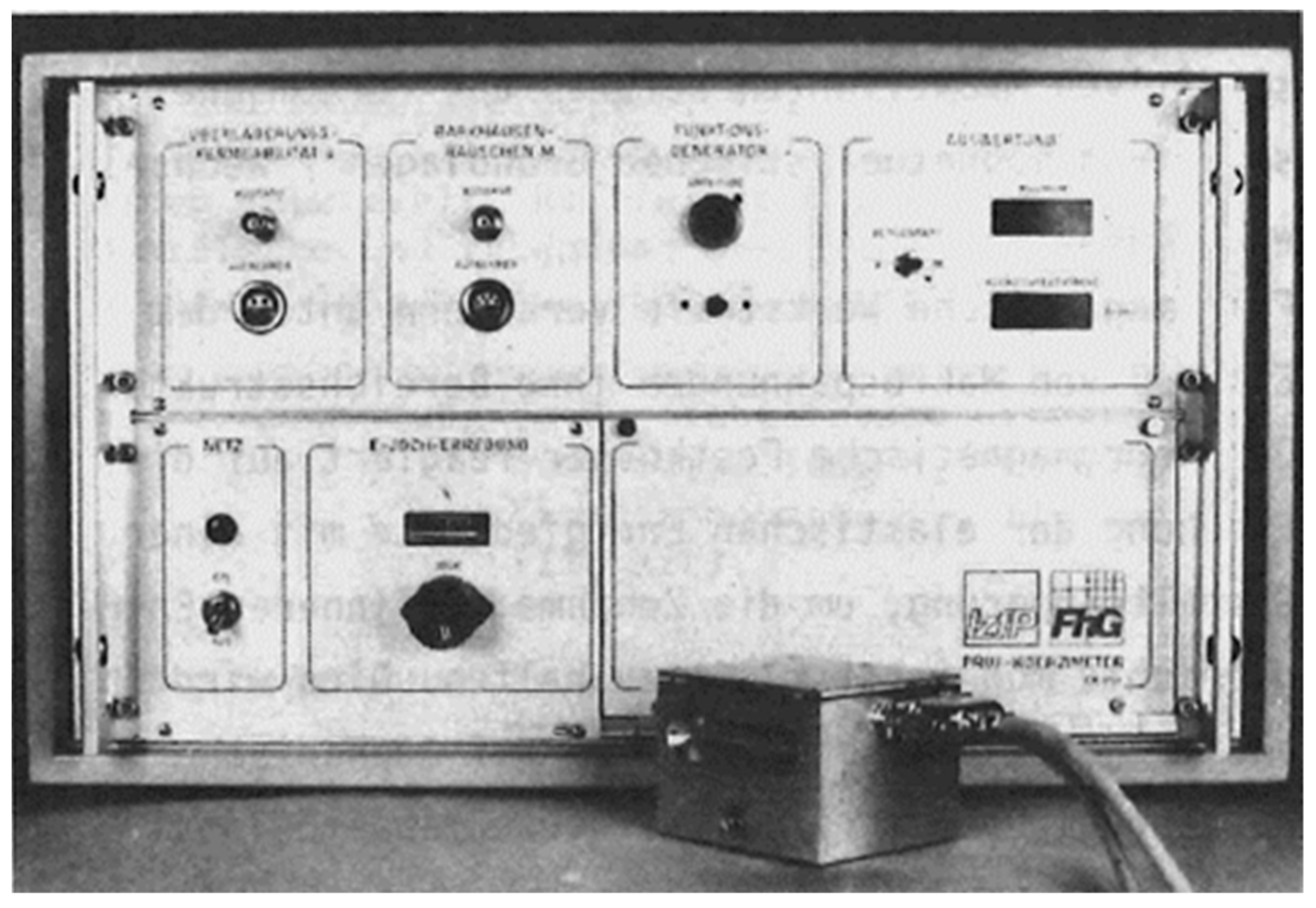
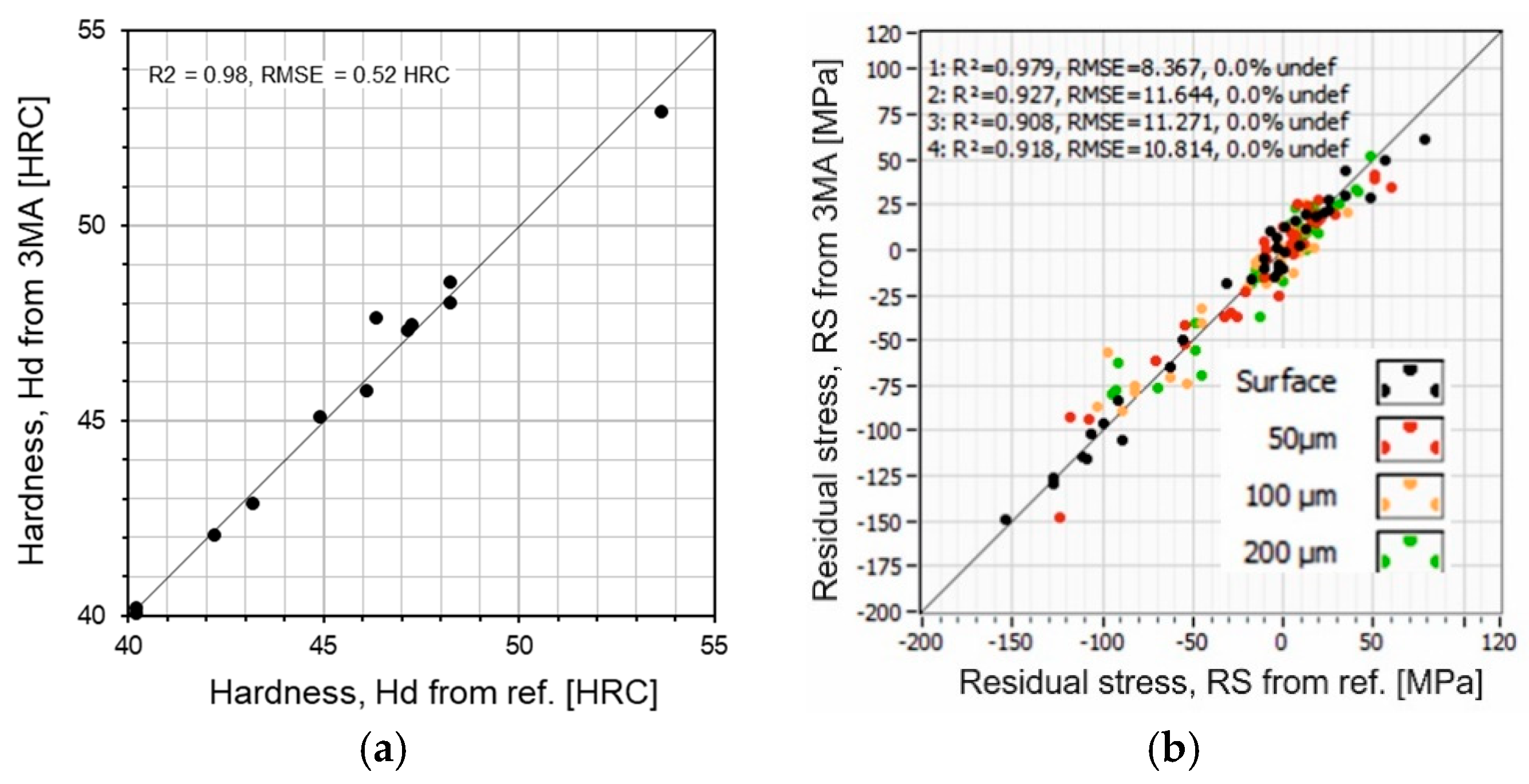
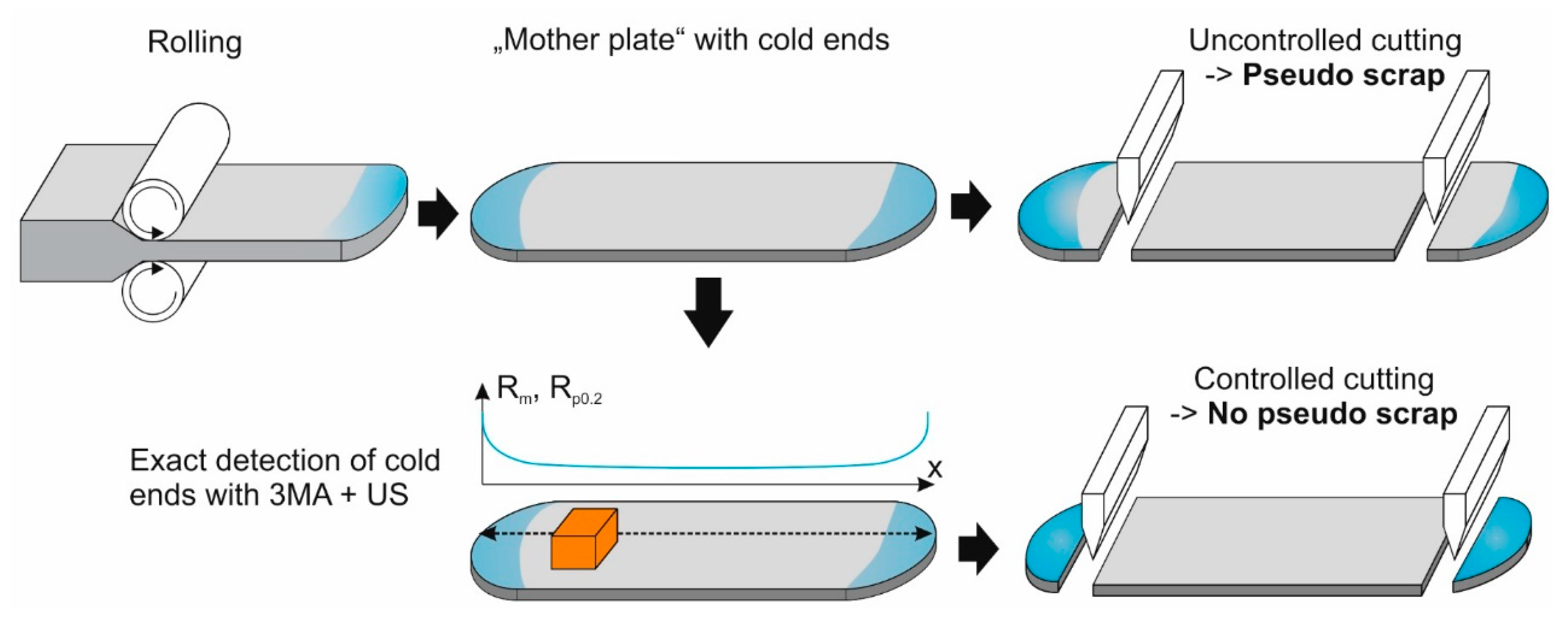
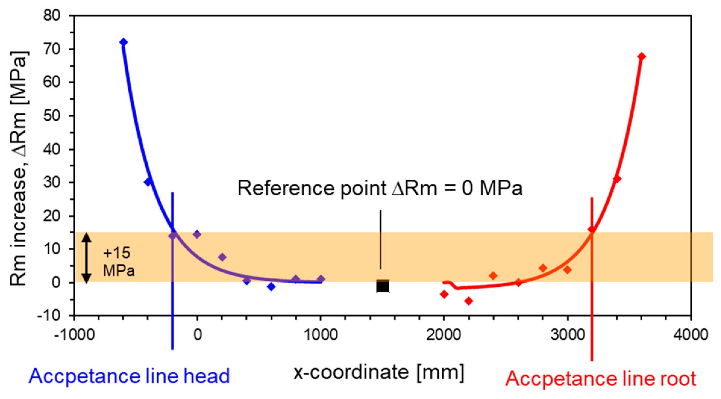
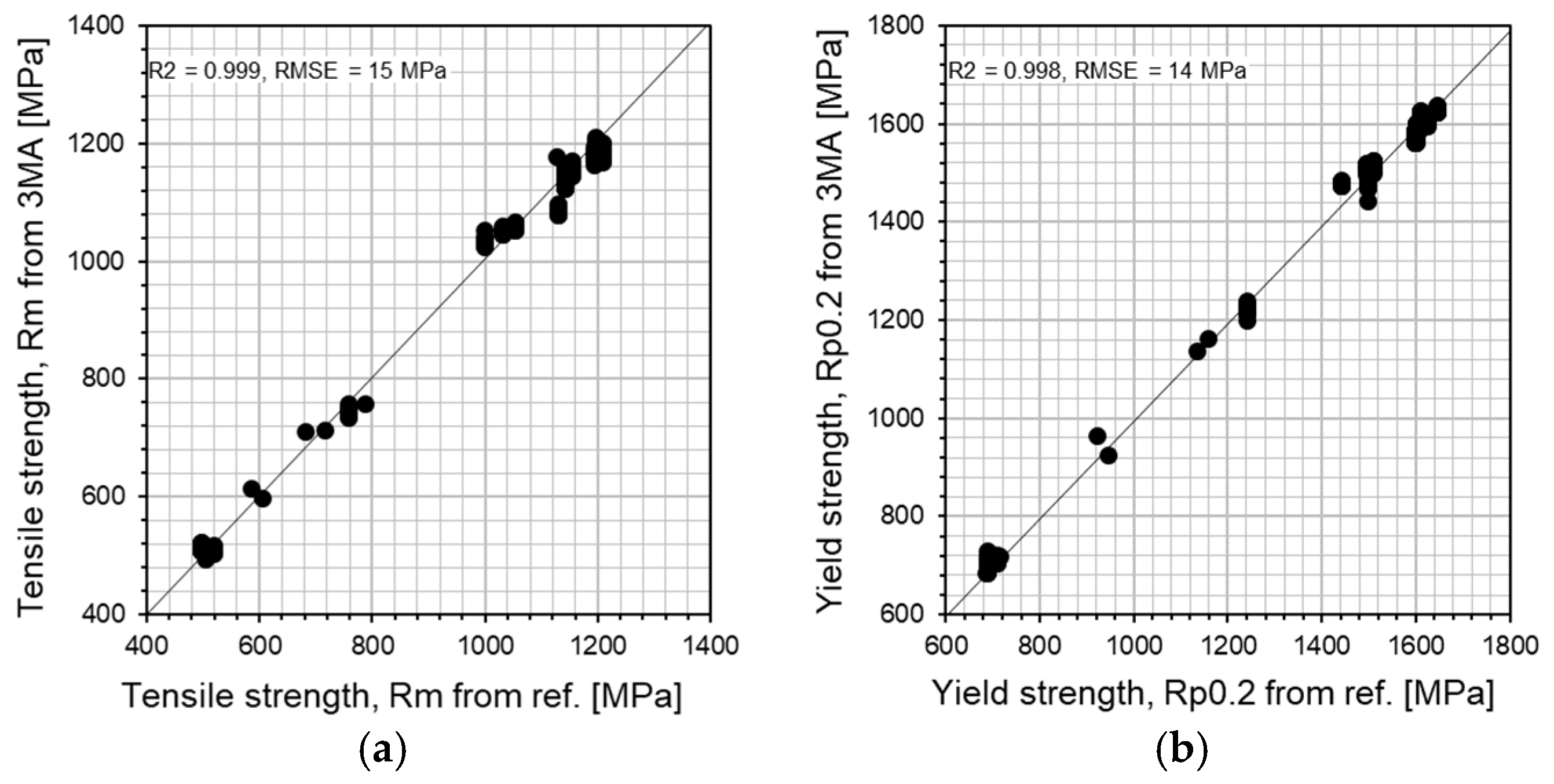
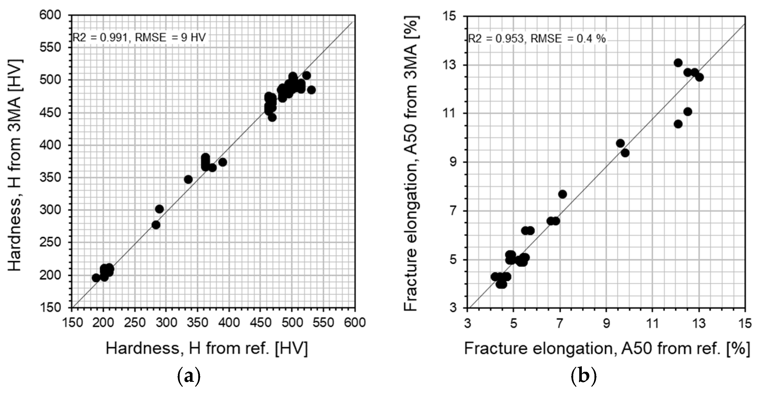
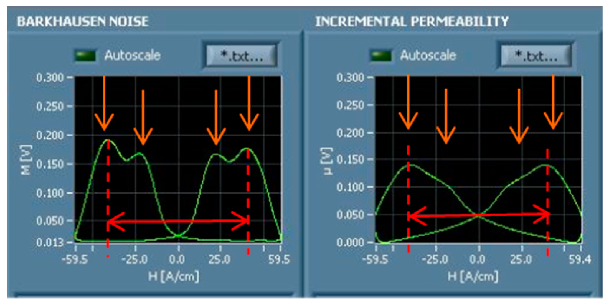
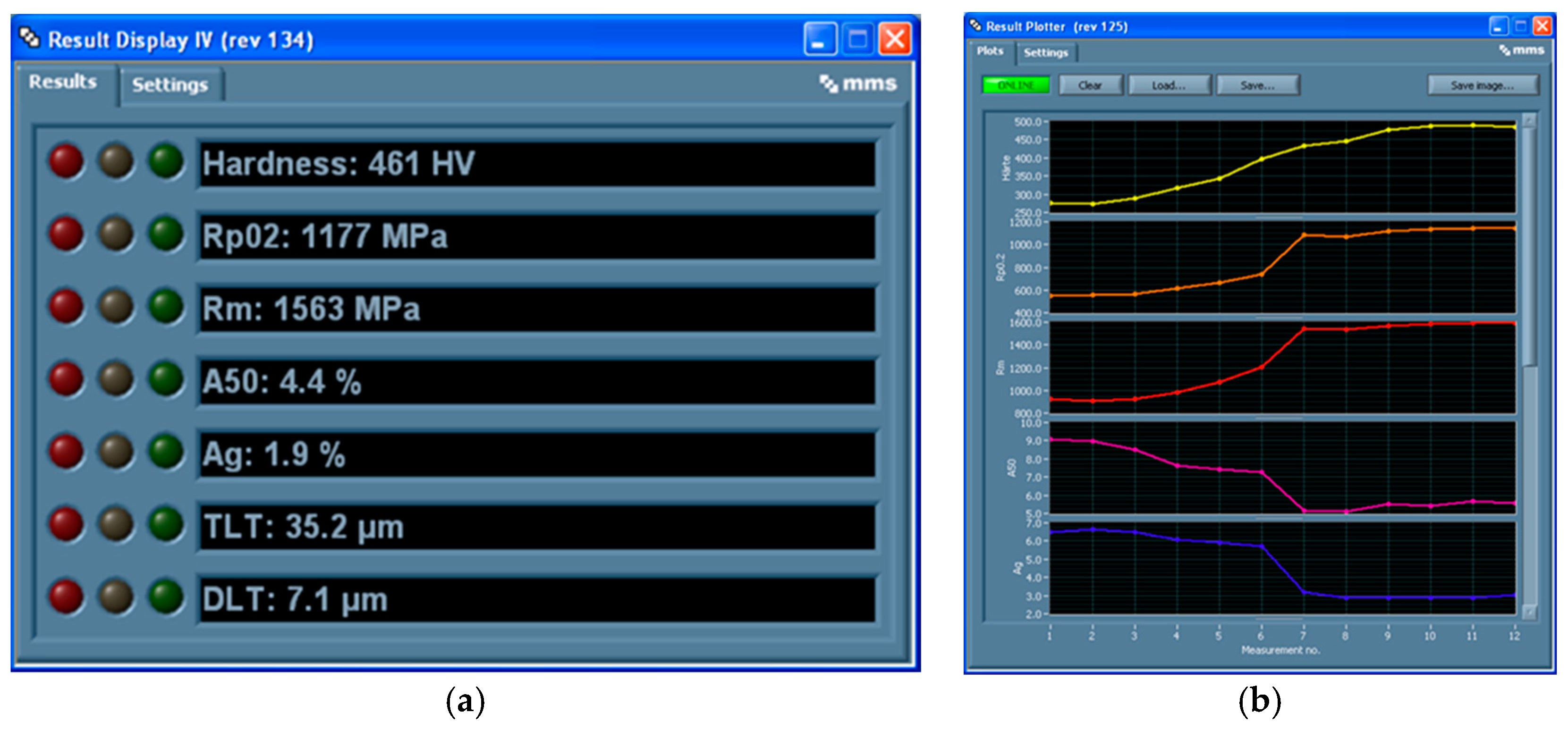
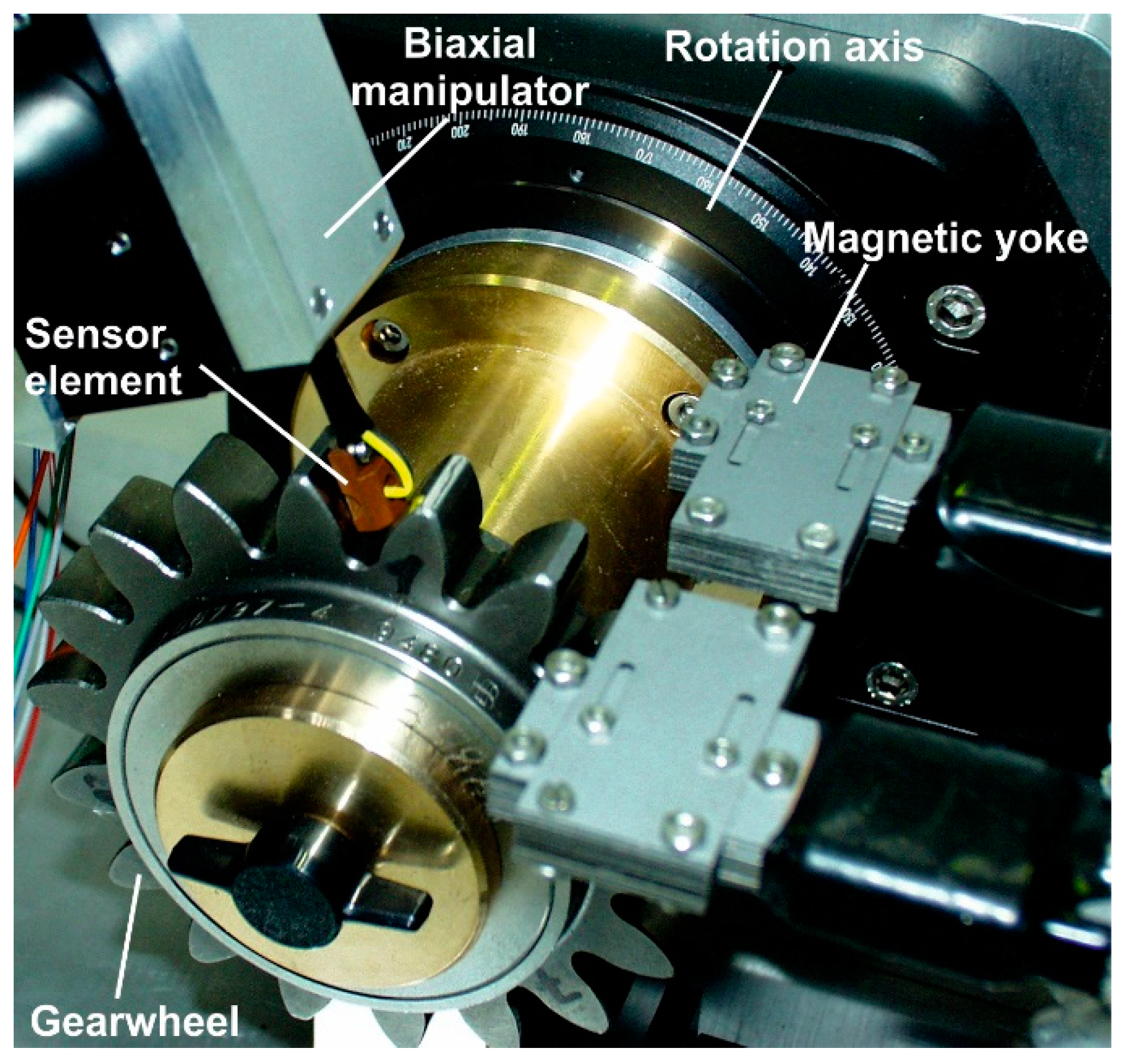
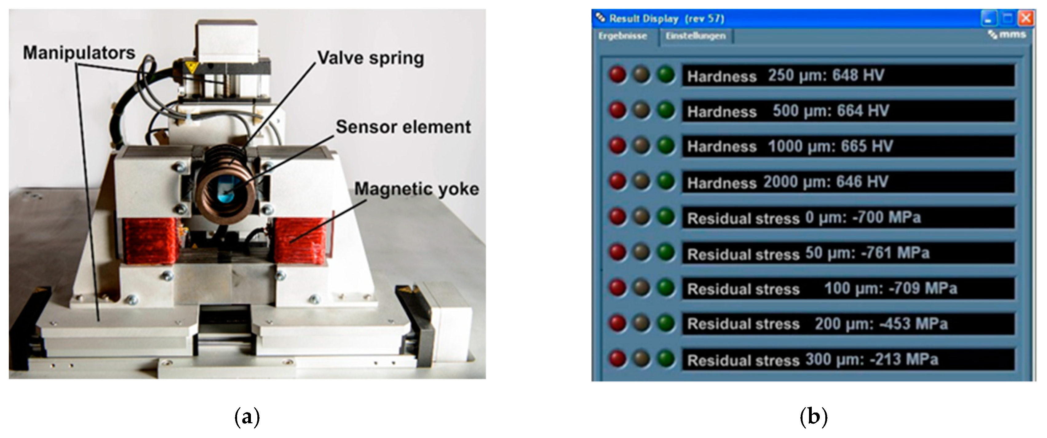
Table 1.
Measuring parameters from Harmonic Analysis (HA).
| Measuring Parameter | Description |
|---|---|
| A1 | Amplitude of the fundamental wave. |
| A3, A5, A7, A9 | Amplitudes of the 3rd, 5th, 7th and 9th harmonics. |
| P3, P5, P7, P9 | Phases of the 3rd, 5th, 7th and 9th harmonics. |
| UHS | Sum of all upper harmonics, |
| K | Distortion factor, |
| HCO | Coercive magnetic field from harmonic analysis |
| Hro | Harmonic content of the magnetic field strength at zero crossing |
| Vmag | Final stage voltage of the electromagnet |
Table 2.
Measuring parameters from multi-frequency Eddy Current (EC).
| Measuring Parameter | Description |
|---|---|
| Re1–Re4 | Real parts of EC signals at frequencies 1, 2, 3 and 4. |
| Im1–Im4 | Imaginary parts of EC signals at frequencies 1, 2, 3 and 4. |
| Mag1–Mag4 | Signal magnitudes at frequencies 1, 2, 3 and 4. |
| Ph1–Ph4 | Signal phases at frequencies 1, 2, 3 and 4. |
Table 3.
Measuring parameters from Barkhausen Noise (BN).
| Measuring Parameter | Description |
|---|---|
| MMAX | Maximum amplitude |
| MMEAN | Amplitude averaged over one magnetization cycle |
| MR | Amplitude at remanence point |
| HCM | Coercive magnetic field, derived from Barkhausen Noise (magnetic field strength at M = MMax) |
| DH25M | Curve width at 25% of MMAX |
| DH50M | Curve width at 50% of MMAX |
| DH75M | Curve width at 75% of MMAX |
Table 4.
Measuring parameters from Incremental Permeability (IP).
| Measuring Parameter | Description |
|---|---|
| µMAX | Maximum amplitude |
| µMEAN | Amplitude averaged over one magnetization cycle |
| µR | Amplitude at remanence point |
| HCµ | Coercive magnetic field, derived from Incremental Permeability (magnetic field strength at µ = µMax) |
| DH25µ | Curve width at 25% of µMAX |
| DH50µ | Curve width at 50% of µMAX |
| DH75µ | Curve width at 75% of µMAX |
Table 5.
Overview of possible 3MA applications.
| No. | Component | Main Application/Description | Ref. |
|---|---|---|---|
| 1 | Components in nuclear power plants | Materials damage and degradation; Neutron-induced embrittlement | [35,36] |
| 2 | Welds (laser, etc.), turbine blades, bearing rings, etc. | Hardness and residual stress | [37,38,39] |
| 3 | Machined parts (gear wheels, etc.) | Thermally induced material damage due to machining | [40,41,42] |
| 4 | Surface hardened or nitrated parts | Hardening depth, depth profiles of hardness and residual stress, retained austenite content | [43,44,45] |
| 5 | Steel grades | Classification of steel grades and microstructure variants | [46,47] |
| 6 | Cast iron | Residual stress, cementite content, primary chill, microstructure gradient | [48,49,50] |
| 7 | Strip steel | Mechanical properties, microstructure features (texture, grain size) and residual stress | [51,52] |
| 8 | Heavy plate and forged parts | Mechanical properties, microstructure features, residual stress, hard spots | [52,53] |
| 9 | Cold formed steel sheets | Residual stress and spring back angle | [54,55] |
| 10 | Hot formed steel sheets | Mechanical properties of steel, coating thickness, resistance spot weld size | [56,57] |
| 11 | Electrical steel | Inspection of cut edges; cutting quality | [57,58] |
| 12 | Miscellaneous | Hydrogen-induced embrittlement, fatigue, toughness, notch impact strength, creep damage | [59,60,61,62] |
Table 6.
Steel grade classes and calibration results.
| Steel Grade Class | RMSE of Rm [MPa] | RMSE of Rp0.2 [MPa] | No. of Strips |
|---|---|---|---|
| IF, conventional | 5.4 | 8.2 | 2667 |
| IF, high strength | 11.3 | 12.3 | 7764 |
| Bakehardening | 5.8 | 8.8 | 1294 |
| Structural | 7.9 | 10.1 | 164 |
Table 7.
Steel grade classes and results of verification measurements for Rm and Rp0.2.
| Steel Grade Class | RMSE of Rm [MPa] | RMSE of Rp0.2 [MPa] | No. of Strips |
|---|---|---|---|
| IF, conventional | 5.3 | 7.4 | 1985 |
| IF, high strength | 6.8 | 9.3 | 68 |
| Bakehardening | 11.2 | 15.6 | 55 |
| Structural | 7.5 | 12.4 | 34 |
Table 8.
Steel grades and results of verification measurements for residual stress.
| Steel Grade | Residual Stress, RS | |||
|---|---|---|---|---|
| At the Surface | At 50 µm Depth | At 100 µm Depth | At 200 µm Depth | |
| RMSE [MPa] | RMSE [MPa] | RMSE [MPa] | RMSE [MPa] | |
| 75Cr1 | 47 | 1 | 3 | 4 |
| 80CrV2 | 15 | 1 | 9 | 31 |
| 50CrMo4 | 4 | 4 | 4 | 11 |
Table 9.
Results of different types of calibration—without and with ultrasound (US) parameters.
| Parameters in Calibration Functions | RMSE of Rm [MPa] | RMSE of Rp0.2 [MPa] | RMSE of Hardness [HB] |
|---|---|---|---|
| Only 3MA parameters | 12 | 23 | 5 |
| 3MA and US parameters | 10 | 11 | 4 |
Table 10.
Results of different types of calibration—without and with US parameters.
| FA0-II | No grinding damage | FB1-II | Light tempered zones at < 10% of the flank |
| FB2-II | Light tempered zones at 10 to 25% of tooth flank | FB3-II | Light tempered zones at > 25% of tooth flank |
| FD3-II | Strong tempered zones | FE3 | Re-hardening |
© 2019 by the authors. Licensee MDPI, Basel, Switzerland. This article is an open access article distributed under the terms and conditions of the Creative Commons Attribution (CC BY) license (http://creativecommons.org/licenses/by/4.0/).
Share and Cite
MDPI and ACS Style
Wolter, B.; Gabi, Y.; Conrad, C. Nondestructive Testing with 3MA—An Overview of Principles and Applications. Appl. Sci. 2019, 9, 1068. https://doi.org/10.3390/app9061068
AMA Style
Wolter B, Gabi Y, Conrad C. Nondestructive Testing with 3MA—An Overview of Principles and Applications. Applied Sciences. 2019; 9(6):1068. https://doi.org/10.3390/app9061068
Chicago/Turabian StyleWolter, Bernd, Yasmine Gabi, and Christian Conrad. 2019. "Nondestructive Testing with 3MA—An Overview of Principles and Applications" Applied Sciences 9, no. 6: 1068. https://doi.org/10.3390/app9061068
Note that from the first issue of 2016, this journal uses article numbers instead of page numbers. See further details here.