Article

A Coupled Evaluation of Operational MODIS and Model Aerosol Products for Maritime Environments Using Sun Photometry: Evaluation of the Fine and Coarse Mode

1
U.S. Naval Research Laboratory, Monterey, CA 93943, USA
2
Space Science and Engineering Center, University of Wisconsin, Madison, WI 53706, USA
3
Department of Atmospheric Sciences, University of North Dakota, Grand Forks, ND 58202, USA
4
U.S. Naval Research Laboratory, Washington, DC 20375, USA
5
Science Systems and Applications, Inc., Lanham, MD 20706, USA
6
NASA Goddard Space Flight Center, Greenbelt, MD 20771, USA
7
Goddard Earth Sciences Technology and Research (GESTAR) II, University of Maryland Baltimore County, Baltimore, MD 21250, USA
8
Département de Géomatique Appliquée, Centre d’Applications et de Recherches en Télédétection, Université de Sherbrooke, Sherbrooke, QC J1K 2R1, Canada
9
European Center for Medium-Range Weather Forecasting, Reading RG2 9AX, UK
10
Japan Meteorological Agency, Tsukuba 305-0052, Japan
*
Author to whom correspondence should be addressed.
Remote Sens. 2022, 14(13), 2978; https://doi.org/10.3390/rs14132978
Submission received: 6 May 2022 / Revised: 8 June 2022 / Accepted: 10 June 2022 / Published: 22 June 2022
(This article belongs to the Special Issue Passive Remote Sensing of Oceanic Whitecaps)

Abstract

:
Although satellite retrievals and data assimilation have progressed to where there is a good skill for monitoring maritime Aerosol Optical Depth (AOD), there remains uncertainty in achieving further degrees of freedom, such as distinguishing fine and coarse mode dominated species in maritime environments (e.g., coarse mode sea salt and dust versus fine mode terrestrial anthropogenic emissions, biomass burning, and maritime secondary production). For the years 2016 through 2019, we performed an analysis of 550 nm total AOD550, fine mode AOD (FAOD550; also known as FM AOD in the literature), coarse mode AOD (CAOD550), and fine mode fraction (η550) between Moderate Resolution Spectral Imaging Radiometer (MODIS) V6.1 MOD/MYD04 dark target aerosol retrievals and the International Cooperative for Aerosol Prediction (ICAP) core four multi-model consensus (C4C) of analyses/short term forecasts that assimilate total MODIS AOD550. Differences were adjudicated by the global shipboard Maritime Aerosol Network (MAN) and selected island AERONET sun photometer observations with the application of the spectral deconvolution algorithm (SDA). Through a series of conditional and regional analyses, we found divergence included regions of terrestrial influence and latitudinal dependencies in the remote oceans. Notably, MODIS and the C4C and its members, while having good correlations overall, have a persistent +0.04 to +0.02 biases relative to MAN and AERONET for typical AOD550 values (84th% < 0.28), with the C4C underestimating significant events thereafter. Second, high biases in AOD550 are largely associated with the attribution of the fine mode in satellites and models alike. Thus, both MODIS and C4C members are systematically overestimating AOD550 and FAOD550 but perform better in characterizing the CAOD550. Third, for MODIS, findings are consistent with previous reports of a high bias in the retrieved Ångström Exponent, and we diagnosed both the optical model and cloud masking as likely causal factors for the AOD550 and FAOD550 high bias, whereas for the C4C, it is likely from secondary overproduction and perhaps numerical diffusion. Fourth, while there is no wind-speed-dependent bias for surface winds <12 m s−1, the C4C and MODIS AOD550s also overestimate CAOD550 and FAOD550, respectively, for wind speeds above 12 m/s. Finally, sampling bias inherent in MAN, as well as other circumstantial evidence, suggests biases in MODIS are likely even larger than what was diagnosed here. We conclude with a discussion on how MODIS and the C4C products have their own strengths and challenges for a given climate application and discuss needed research.

Graphical Abstract

1. Introduction

Over 70% of the Earth’s surface is ocean, and by its very nature, the marine environment is a dominant component of the climate system. However, this coupled aerosol, ocean, and atmosphere system is particularly difficult to monitor consistently over the globe. One of the fundamental challenges to understanding the remote marine environment is related to the significant sensitivity of clouds to the presence of cloud condensation nuclei (CNN). Wind-driven coarse and fine particles, as well as secondary production from marine emissions, were long thought to help regulate global climate through direct and indirect feedback [1]. However, because terrestrial aerosol emissions and CCN can be transported extraordinary distances, they were counter-hypothesized to dominate cloud radiative budgets in even the most remote marine regions [2,3,4,5]. Given the relatively low concentration of aerosol particles in baseline marine boundary layers, even small terrestrial contributions to the CCN budget can potentially have significant cloud impacts. For example, systematic differences in CCN populations and cloud properties exist between more terrestrial-influenced northern oceans versus southern oceans [6]. Beyond general findings, the climate and operational aerosol communities still struggle with aerosol attribution and climate feedback in marine environments [7,8,9,10].
The sensitivity of clouds to CCN places demands on the community’s ability to monitor and simulate the remote marine environment. Field data can offer the most comprehensive set of measurements with high accuracy, but in situ observations inherently represent a local environment in time and space that can be strongly influenced by oftentimes unconstrained upwind processes. Further, studies often utilize different instrumentation and measurement protocols and generate data of differing quality, thereby making quantitative comparisons difficult. For global monitoring the community must rely on a combination of remote sensing and modeling products. Additionally, even the aforementioned field measurements often must utilize such products to interpret local data. Remote sensing offers near-global observing, but with significantly less local information content, strong scale dependencies [11], well-documented biases [12,13,14], and, at times, an associated clear sky sampling bias [15]. Models can provide complete 4D simulations with detailed physics and source information, but physics is parametrized and can be sensitive to even slight changes in sources and environmental conditions. Uncertainty in physics and sensitivities to the environment still lead to large differences in outcomes in free model simulations [16]. The subsequent tuning of models or the utilization of data assimilation of bias-corrected satellite data in operational aerosol models has moved simulations closer to available observations. However, in doing so, modelers risk not only a disconnect from the real physics but changing the wrong parameter to achieve closure.
Aerosol Optical Depth at 550 nm (AOD550) and its fine mode fraction (η550) are perhaps the most tractable and informative remote sensing products for maritime aerosol monitoring, as these are the parameters that span observations to models and are easily available at relatively high accuracy. The simple Ångström Exponent (AE) that describes the wavelength dependency of AOD is also popular. However, the Ångström Exponent is degenerate in size and modal contribution relative to more tractable physical attributes such as the fine and coarse mode optical depth [17,18,19]. Indeed, both physical and remote sensing optical models typically (although not universally) use bimodal number or volume distributions with fine and coarse mode components (examine [20,21,22] and references therein). To first order, coarse mode contributions to AOD550 (or CAOD550) can be attributed to sea salt and dust. Likewise, fine mode contributions to AOD (or FAOD550) are associated with biomass burning, anthropogenic pollution, or natural primary (including marine) and secondary particles. Such AOD components, while adding a much-needed degree of freedom, are nevertheless unsatisfying for estimating aerosol particle mass or CCN concentrations as they comprise an integrated bulk metric within a four-dimensional, cloud-dominated, and high humidity environment. AOD uncertainty and its transformation into microphysical quantities such as number or mass are particularly difficult in regard to cloud adjacency (e.g., see [23] and references therein). AOD components only partially project on what the community wishes to know, namely sources, mass concentrations, numbers/CCN concentrations, size distributions, chemical compositions, and local radiative impacts, particularly in the marine boundary layer (MBL). However, AOD components are what the community largely has available, both in terms of coverage and accessibility.
To meet the challenge of global aerosol monitoring and estimate key geophysical quantities, remote sensing products and models are now commonly merged within the data assimilation construct. Aerosol models are updated with available remote sensing observations, typically the one global observable, AOD. However, the data assimilation process should not be seen as simply updating the model to match available AOD. Data are first rigorously quality assured and bias-corrected, then for each of the myriads of assimilation methods (e.g., 2D var, [24]; 3D and 4D var, [25]; and ensemble Kalman filter, [26]), detailed procedures on how the model should be adjusted to closely match the observations are applied. Adjusting the model to observations, which naturally leads to a closer model representation of the observations, may very well result in either improvement or worsening of errors in individual model components. Uncorrected errors in those observations likewise lead to downstream errors in the simulation. Thus, for data assimilation, one of the significant challenges is understanding and correcting the observational error.
As models and remote sensing products are gradually being combined in research [27,28], it is anticipated that coupled analyses will become a tool that is increasingly used in the community. This paper provides a comparative analysis of 550 nm AOD550, η550, and corresponding FAOD550 and CAOD550, from the perspectives of the two global operational products: (1) the Moderate Resolution Imaging Spectroradiometer (MODIS) Version 6.1 dark target (DT) aerosol retrievals (henceforth MODIS DT provided within Level 2 product known as MOD04/MYD04; [29]); (2) the corresponding consensus speciated AOD products drawn from International Cooperative for Aerosol Prediction Multi Model ensemble (ICAP-MME; [30,31]) with members that utilize MODIS total AOD in assimilation (i.e., generating the so-called “core four consensus” or C4C of the ICAP-MME). Currently, operational models assimilate Terra and Aqua MODIS’s total AOD550 but not FAOD550 and CAOD550. MODIS and C4C products are compared to one another, with discrepancies informed by the Marine Aerosol Network (MAN; [32,33]) collection of shipboard sun photometer data, with further evaluation from isolated island sites from the Aerosol Robotic Network (AERONET; [34]).
In order to understand remote marine environments, it is necessary to collectively consider the baseline uncertainties of remote sensing observations and models simultaneously, especially in the pristine conditions where signals are low, and aerosol-cloud relationships may be most sensitive to aerosol intrusions (e.g., from terrestrial sources). Indeed, while basic error statistics for maritime MODIS DT and the C4C have been presented in many previous works (cited within this paper), we distinguished this work by (1) focusing on the fine versus coarse partition of AOD550, (2) examining their spatial biases and covariances, and (3) producing magnitude dependencies, as opposed to the regression-based analyses over a few sites that are typically performed. After providing a baseline analysis, a set of additional contextual analyses, including satellite quality assurance, cloud fractions, and regional investigations, are presented. From this point, several questions are addressed: (1) Are there any notable measurement, retrieval, and modeling inconsistencies in AOD components? (2) Are these differences consistent with known issues in the literature? (3) What is the promise of assimilating MODIS 6.1 modal (i.e., fine, coarse) products for improving the global model representation of the marine environment? (4) Are there any obvious corrections developers can make or further hypotheses to be investigated to improve product skill or representativeness?

2. Methods, Data, and Models

The evaluation strategy in this work is to examine operationally generated MODIS and ICAP C4C products to help inform the next generation products of the Earth-observing and simulation systems. The operational products were evaluated here in a manner consistent with their advertised use in the scientific community. The period of study for this investigation is the four calendar years from 2016 to 2019. An evaluation of the ICAP-MME C4C consensus product against land-based AERONET derived AOD550, FAOD550, and CAOD550 was previously conducted for this time period, and the C4C was shown to have superior and largely uniform skill in time compared to the individual contributing models, even with periodic model updates [31]. The year 2020 was excluded due to atypical maritime conditions, including Australian pyroCB activity that generated a southern hemisphere stratospheric smoke layer with persistent and above-average AOD values for approximately 4 months, and potential COVID-related inconsistencies in aerosol emissions [35,36].

2.1. MODIS

Version 6.1 of the MODIS Dark Target Algorithm (MOD04/MYD04) is one of the most utilized and evaluated satellite-based aerosol products in the community, due in part to the association of Aqua MODIS with the A-train. MODIS DT gives near-global daily coverage, and for the marine environment, its AOD and Ångström Exponent products were exhaustively evaluated against cloud contamination, whitecaps, near-surface bubbles, etc. [29,37,38,39,40,41,42]. These studies also show that identified shortcomings in the marine component of MODIS Collection 5 and its predecessors were reduced or eliminated in the current MODIS Collection 6.1. However, residual biases remain. For example, the global error in AOD550 is (+0.04 ± 0.1 × AOD550) to (−0.02 + 0.1 × AOD550) [29], which is suggestive of a mean bias of +0.02. In this same study, while no specific error bar was provided for the 550 to 870 nm Ångström Exponent, the variation was given, and results indicate a clear positive bias in Ångström Exponent for lower AOD550 values (e.g., Figure 17 of [29]). However, no specific error bar was given other than 68% of data falls within ±0.41. In comparison, mean ocean AOD550 was listed as 0.150, 0.135, and 0.155 for Terra MODIS DT, Aqua MODIS DT and Multi-angle Imaging Spectroradiometer (MISR) [40].
The operational dark target product is derived using separate over land and over ocean algorithms [29]. Water is strongly absorbing in the red and near-infrared and, as a result, is the most ideal lower boundary condition for maximum information extraction. Nevertheless, it is necessary to account for wind-driven whitecaps, shallow water, and heavy sediment loads. The ocean algorithm uses six MODIS observed radiances (0.55, 0.65, 0.86, 1.24, 1.63, and 2.11 μm) and a set of fine and coarse mode aerosol models in a lookup table to retrieve spectral AOD and fine mode fraction. Masks are applied for clouds, as well as for shallow water and sediment, and cloud fractions are derived. Retrievals of AOD550, FAOD550, CAOD550, and η550 are based on the 10 × 10 aggregates of 1 km native nadir pixels, resulting in nadir retrieval sizes of 10 × 10 km and an edge of swath retrieval size of approximately 50 × 30km. For this analysis, AOD components were extracted and aggregated with center points on a 1 × 1 degree grid to match the ICAP-MME C4C described in Section 2.2. A 3 km MODIS DT product is available but was found to have lower accuracy than the standard product evaluated here [43]. It is noteworthy, based on simple scan geometry and the presence of sun glint, that samples are skewed towards the edge of the scan versus the center. For example, for the 1 × 1 degree match-ups with MAN, the 25%, 50%, 75%, and 100% quartiles for scan zenith angle for Aqua MODIS samples are 30°, 45°, 57°, and 65°.
Several studies were undertaken to investigate the sensitivity of the presented results to data aggregation. Investigated factors included the aggregation pixel size, the temporal window, quality assurance flags, inclusion or exclusion of negative AOD retrievals, and cloud fractions. MODIS DT products have quality “confidence” flags ranging from 0 to 3, which correspond to poor, marginal, good, and very good confidence in their quality. Confidence is assigned based on a number of metrics, including the number of non-cloudy pixels, relative proximity to glint, observation/lookup table fitting errors, etc. As a matter of operations, data with a flag of 0 are typically not used, with previous studies suggesting that flags 1 through 3 are acceptable. As no flag 2 data were present in the dataset, all data with flags 1 and 3 were aggregated together. In the current study, error statistics were recompiled for data aggregation of flag types 1 and 3 separately, noting that in a 1 × 1 box, there is a mix of qualities present for any given data point, and data aggregation and distillation are a necessity in research. While the focus of this work is on the commonly used level 3 MODIS products that are used to support global monitoring, data assimilation, and verification, data aggregation leads to a potential loss of information. As a result, an adjustment of the data aggregation window was also conducted. Additionally, special attention was paid to other sampling factors, including cloud fraction. Specific investigation findings included:
(1)
QA flags: QA flags in the range of 1 (marginal) and 3 (very good) did not alter our findings. Therefore, both data flags are suggested for use in order to include the largest number of data points. As a matter of procedure, data flag 0 (low confidence) data were not examined. A flag of 0 indicates an internal inconsistency in the retrieval or that the scene was in glint or had too few “clear/non-cloudy” pixels for higher confidence. Elevating data points from a flag 0 to a flag for acceptable use is left to another investigation;
(2)
Aggregation size and temporal window: Aggregations were reduced to +/−0.25 degrees and +/−1 h. Under most circumstances, this allowed for only one or two retrievals to be aggregated. Restricted windows resulted in a 70% loss of the data matches and did not change the study findings;
(3)
Negative retrievals: The MODIS DT retrieval allows for negative AOD outcomes. Individual negative level 2 retrievals were found to account for 0.1% of all retrievals, and their inclusion or omission did not alter the study findings;
(4)
Geometry: Biases reported here are largely not dependent on scattering or scan angle. The expectation was a ~+0.05 high bias for the 50 points where scattering angles were >170° (i.e., backscattering), but little change in RMSD. These are not enough points to change any reported number. This does not mean that such dependencies do not exist, but they are not statistically significant in comparisons to MAN.
For completeness, the over-land MODIS combined Dark Target/Deep Blue (DT/DB) product is included in some figures, as well as a short analysis [37]. Given the complexity of the land surface as a lower boundary condition compared to dark water, the MODIS AOD over land algorithms are significantly different from their over-ocean counterparts. The MODIS DT/DB data field is populated with the over-land product that is best suited for a given land surfaced type. For example, Dark Target is used for forests while Deep Blue is used for arid environments. Given the seasonality of surface albedo, the contributing product for a given location can change by month. While the DT/DB is useful for total AOD550, there is no fine mode fraction operationally generated.

2.2. ICAP-MME C4C Model Products

The ICAP-MME provides a reliable community baseline for evaluating aerosol prediction performance. The utility of using the ensemble mean (i.e., a consensus) as a baseline was demonstrated for various community prediction capabilities (e.g., forecasters [44]; coupled models [45]; tropical cyclones [46]; climate change [47], and so forth). The C4C is generated from 6 hourly speciated global model AOD fields, including fine and coarse mode, delivered daily by the following modeling systems: (1) Copernicus Atmosphere Monitoring Service (CAMS; [25]); (2) the Japan Meteorology Agency (JMA) Model of Aerosol Species IN the Global AtmospheRe (MASINGAR; [48]); (3) the NASA Goddard Earth Observing System (GEOS; [49]); (4) the US Navy Aerosol Analysis and Prediction System (NAAPS; [50]). Each C4C contributing member uses operational numerical weather prediction (NWP) meteorology, carries multiple aerosol species, and assimilates MODIS v6.1 AOD550-related products for generating initial forecast conditions. A description of these systems, the formation of the consensus, and evaluation against AERONET sites are all provided in the literature [30,51]. Each model system has its own methodology for preparing, quality-assuring, and assimilating data. CAMS, MASINGAR, and NAAPS quality-assure, bias-correct, and aggregate the MODIS dark target AOD550 product prior to assimilation. GEOS utilizes the aggregated radiances used in the v6.1 retrieval and applies its own neural network retrieval to generate an AOD550 product for assimilation. A key finding is that while each C4C member has its own strengths and weakness by region and or species, the C4C consensus provides better and spatially more consistent AOD550 aerosol guidance than any of the individual contributors over the entire globe [30,31,51]. Additionally, both of these papers also show that the C4C universally underestimates AOD550 for significant events. As is shown in this evaluation, these findings hold true for the maritime environment. As with many other models, the models contributing to ICAP were tuned by their developers to match available observables, and due to both coverage and skill, MODIS DT v6.1 MOD04/MYD04 AOD550 is the dominant observation.
The advantage of the ICAP-MME C4C, relative to climate or other forms of free-running model simulations, is that it combines the output from several independent meteorologies and aerosol models that make use of data assimilation, which pulls the resulting meteorological and aerosol states towards the assimilated observations. The disadvantage of the C4C is that each of these contributing models, as does any operational system, undergoes periodic updates, leading to shifts in the input of the consensus. However, such changes are often limited and balanced out by changes in the performance of the other models. It should also be noted that all four models have a closely related reanalysis counterpart that allows for future ICAP-related reanalysis consensus AOD550 products, expected in the next few years. In the meantime, model variability is overcome by focusing the study and its conclusions on the relative differences between the model consensus and MODIS DT, with differences adjudicated by comparison to the “ground-truth” MAN and AERONET observations. Through the presented analysis, consistent biases between the models, MODIS retrievals, and the sun photometer observations are shown. As agreed upon by the ICAP-MME model developers, the skill scores of the individual contributing models to the C4C are not disclosed. However, anonymous similarities and differences across the models in the form of model spread are discussed.
The presented analysis used the official ICAP consensus product in which AOD mean and standard deviation were generated by re-gridding model fields with different resolutions onto a standard 1 × 1 degree grid. The consensus was created with the 0Z model run, which includes a 0Z analysis and forecasts out to 18 h. By using the 0Z runs, the Pacific benefits from data assimilation at the analysis time while, for example, the Indian Ocean and Atlantic utilize a ~6 h and 12 h forecast, respectively. The use of short-term forecasts in the evaluation is necessary for 6, 12, and 18Z. While all of the contributing centers consistently generate and post a 0Z analysis field, this is not the case for the 6, 12, and 18Z analyses; therefore, forecasts are used instead. While each model in the C4C has different resolutions, physics parametrizations, aerosol size bins, driving meteorology, and data assimilation schemes, one consistency is that they each assimilate Terra and Aqua MODIS total AOD550 products. None of the contributing models assimilate aerosol size-related observations such as η550, FAOD550, CAOD550, or Ångström Exponent at this time. Therefore, the projection of total AOD onto model aerosol species concentrations is based on the individual model and data assimilation systems, which most often conserve some prior aerosol speciation in the updated analysis.
An important consideration in the C4C is that each contributing model has differences in its representations of aerosol size distributions and speciation. While “total AOD” is a universal observable that can project onto and be used to tune each model quite easily, applying fine and coarse aerosol observations to the individual models is dependent on the speciation and size representation that are chosen by the model developers. As each ICAP model is uniquely configured, there is no universal definition and modeling methodology for describing size. All of the C4C models have some combination of “bulk” single mass and size-resolved species. For example, the NAAPS model is a complete bulk model that attributes a single mass bin for each of the four represented species, all based on the aerosol source (dust, sea salt, biomass burning smoke, and a combined anthropogenic/biogenic fine). Other contributing models carry aerosol particles by their chemical composition (e.g., organic carbon, sulfate, black carbon, etc.), which come from a combination of sources. The aerosol particles by composition are represented by several size bins. For example, GEOS-5 carries five dust and sea salt size bins, two bins of BC and OC, and one bulk bin for sulfate. CAMS carries three sizes for dust and sea salt and bulk for other types. Finally, MASNGAR has ten-size bins for dust and sea salt but treats BC, OC, and sulfate in bulk. Given these differences, it was necessary to define FAOD550 and CAOD550 in a manner that was achievable across the contributing models and could be verified in a similar manner as the previous evaluation studies [30,52]. First, all combustion and biogenic sources (sulfate, OC, BC, ABF, biomass burning) are defined by the models as fine mode-whether bulk or, in the case of GEOS-5, having only two sub-micron size bins. Thus, AOD from these species can be summed to derive a fine mode AOD. The coarse mode is more complicated. While sea salt and dust production have a dominant coarse mode (with a mass median diameter on the order of 5 μm), there is nevertheless production at sub-micron diameters at the lower tail of the overall mass distribution. For evaluation purposes, we assigned such submicron particles to the coarse mode as they are part of the overall coarse mode production distribution. This is comparable to how it is handled in MODIS and the MAN data, as described below. This is a reasonable approximation since the total AOD contributions are small compared to the super-micron portion of the distribution, as evidenced in the spectrally flat nature of their AOD spectrum described below. Nevertheless, these definitional considerations were discussed throughout the analysis presented in this work. Ongoing work by some of this paper’s authors is further quantifying such uncertainties.

2.3. Maritime Aerosol Network (MAN) and Aerosol Robotic Network (AERONET)

The principal evaluation dataset to explain differences in the MODIS and C4C is from the MAN network of hand-held sun photometers. MAN is a maritime counterpart to the Aerosol Robotic Network (AERONET; [34]), developed to support research cruises and other remote observations where a standard Cimel sun photometer is not feasible [32,33]. Currently, the MAN network is the only reliable source of global maritime AOD verification data in large numbers. An advantage of MAN over terrestrial-based AERONET is its coverage for true maritime conditions. While AERONET does include some remote locations, these are typically located on the leeward side of the islands’ prevailing winds (where research stations are often located). Coastal sites are regularly influenced by continental or island sources or littoral meteorology. Further, shore-based sites with predominantly onshore flow exhibit perturbed boundary layers and local flow circulations [53]. Thus, the set of available AERONET sites for this analysis is quite limited, and few are located adequately to inform product biases. Given such limitations, six island AERONET sites were selected to examine the consistency of the MAN results. Descriptions of AERONET data are available in many papers [34,54,55] and are, therefore, not duplicated here. However, given the reliance on MAN data in this study, some description is required. For MAN, Microtops sun photometers are distributed by AERONET with GPS units and are pre- and post-calibrated for research cruises throughout the world. Instruments come in various configurations with channels spanning 340–1020 nm, with the potential for including aerosol, ozone, and water vapor channels. All of the data utilized in this work include successful 440, 500, 675, and 870 nm measurements. The MAN handheld sun photometers are calibrated against the AERONET reference instruments, which are in turn calibrated by the Langley method at the Mauna Loa Observatory, yielding a reference instrument accuracy of ~0.005 or less (excluding the UV channels; [56]). An estimate of the MAN AOD uncertainty based on shipboard observation field data is ~0.02 [32], while the AOD uncertainty for the AERONET field measurements is ~0.01 in the visible through near-infrared and ~0.02 in the UV [56]. MAN products share AERONET nomenclature: Level 1 (not cloud screened), Level 1.5 (cloud screened), and Level 2 (cloud screened and post calibrated). However, due to the handheld nature of the MAN instruments, cloud screening procedures are different.
Standard AERONET and MAN products include spectral AOD, 440–870 nm Ångström Exponent, column precipitable water vapor, and 500 nm Spectral Deconvolution Algorithm (SDA; [18]) derived fine/coarse mode AOD fractions. For this work, both MAN and AERONET fine and coarse mode AOD were also extracted using SDA, but the code was modified to extract a benchmark wavelength of 550 nm as verified with in situ maritime data by [19]. In defining fine mode fraction, the SDA optically (spectrally) accounts for the full modal distributions of the fine and coarse modes: the AERONET version of the SDA relies on the presence of (independent) modal distributions whose 2nd order spectral signatures are optically distinguishable. Thus, fine mode particles associated with the tails of the overall coarse mode distribution are assigned to the coarse mode and vice versa. This is similar in nature to the aforementioned remote sensing optical and numerical prediction models, which have fine and coarse mode aerosol distribution representations. This is also the case for the aerosol species represented in the ICAP-MME models. However, it is noteworthy that much of the verification of the MODIS η550 product was performed using the Dubovik and King [57] retrievals on AERONET almucantar data (e.g., henceforth DK). The DK makes a distinction between fine and coarse mode not based on the full lognormal distribution of each mode but rather based on the diameter nearest to the minimum of the retrieved particle-volume distributions selected from four specific AERONET diameter bins. Typically this point is ~0.8 μm in diameter. Because fine mode distributions tend to narrower geometric standard deviations than the coarse mode, such definitional differences would result in a slightly higher η550 in DK than SDA for mixed fine/coarse environments. A bias would then manifest itself against fully modal fine and coarse mode optical models. The topic of the interpretation of modal optical properties is the subject of ongoing studies by this paper’s authors (e.g., O’Neill et al. and Reid et al., currently being written). Overall, the SDA and the DK results are exceptionally well correlated for FAOD550, CAOD550, and η550 (r2 > 0.98 on all accounts). However, DK does provide η550 values higher than about 0.05–0.1 for 0.3 < η550 < 0.7, while the DK/SDA differences converge to near zero for fine-dominated environments. It should be emphasized that the comparison of MODIS, C4C, and MAN data, as outlined here, are more consistent using the SDA. The importance of these differences was discussed periodically in this paper.
A total of 14,226 level 2 MAN data points were used in this study. Each data point is in fact, derived from up to 20 measurements within a short period of time, from which the spectral AODs are calculated based on the maximum solar radiance observed from this period. Since a human operator (especially in heavy seas) may not point exactly at the sun (leading to biased-low measured radiance and biased-high derived AOD), these multiple measurements help to ensure at least one of highest quality. Data collection frequency (e.g., individual data points posted by MAN that aggregate these samples from each measurement) varied considerably by operator and conditions. Most often, a single data point (derived from a collection of high frequency sampling) would be collected in an hour, but sometimes up to thirteen were made (separated by longer gaps). In order to normalize, all data were processed into hourly data averages and standard deviations, producing 8637 independent hourly data points. These points and their AOD550 values are provided in Figure 1a. Of the data points, 5638 (65%) were isolates (one complete data collected within that hour), 1566 (18%) had two observations, 786 had three (9%), and so forth. MAN data reports an uncertainty in AOD of ±0.02. Data within aggregates were also stable, with standard deviations for aggregates averaging 0.008 ± 0.01 and with the largest fractional outliers being associated with extremely low AOD550 (<0.05). This consistency is in part due to the quality assurance practices that elevate data to level 2, including the manual removing of data by MAN for significant outliers.
Just as with terrestrial AERONET deployments, MAN data collecting is influenced by a combination of scientific needs with cruise availability and weather opportunities. Thus, MAN observations have inherent sampling bias. As a result, MAN observations were utilized to evaluate biases and local error in MODIS and the C4C rather than relied upon to make a definitive statement about climatological values in the global marine environment (unlike some fixed AERONET sites with decadal data records). Inspection of the global distribution of MAN samples (Figure 1a) shows a very similar pattern to the original 2004–2010 period of MAN [32], with the current dataset having more opportunities in the more remote oceans. Observations are predominantly near coastal regions because it is in these areas that research cruise frequencies dominate, especially for smaller research vessels. The Atlantic Ocean and the Mediterranean Sea display many cruise transects from Western Europe to offshore western Africa and down to the southern tips of South America and Africa. A second set of tracks populates western Africa through the Caribbean. These cases are largely due to an interest in African dust. Not surprisingly, high AOD550s (e.g., AOD550 > 0.2) are generally in the tropical to subtropical belts, with the highest values being for dust off of western Africa, dust and pollution over the Red Sea/Arabian Gulf, pollution over East Asia, and biomass burning from central Africa and the Maritime Continent. Likewise, the lowest AODs are over remote oceans.
MAN observations are taken when deemed appropriate by the operator. As is shown in this work, operations results in a clear sky selection bias in regions with high storm prevalence, such as the southern oceans. Also, difficulty in pointing a hand-held sun photometer in heavy seas could lead to sampling bias when sea salt concentrations are expected to be the highest (e.g., a clear-sky bias in stormy regions such as the southern oceans with few observations of windblown sea salt). As part of this study, findings are cross-compared to the limited data available at six AERONET sites in Section 4, which are shown to be largely consistent to MAN findings. Nevertheless, because of inherent sampling bias in the systems, we emphasized that verification statistics should not be considered climatological (e.g., describing the absolute magnitude of overall global value or bias in the products) but rather help inform the locations and the relative magnitudes of biases for future correction. This work leads to the development of a next-generation set of error models so that less biased analyses can be generated.
While global aerosol features are visible in Figure 1 (e.g., African dust, subtropics, Asian outflow, etc.), MAN also demonstrates how pristine the oceans are, even when a large fraction of the samples are coastal and targeted for polluted environments. Figure 1b provides a cumulative log probability plot of AOD550 for all samples, and fine and coarse AOD550 from SDA. Median MAN AOD550, FAOD550, and CAOD550 for this sample are 0.08, 0.03, and 0.05, respectively. Therefore, unsurprisingly, the maritime environment is coarse mode dominated in this dataset. Given MAN samples from numerous sources, the data distribution is only moderately lognormal (e.g., a true lognormal distribution would be a straight line in log–log space). Population-wise AOD550 percentiles 16%, 50%, 67%, 84%, 95, and 99% correspond to values of 0.034, 0.08, 0.12, 0.28, 0.5, and 0.8, respectively. This leads to an overall median value of 0.08 and a geometric standard deviation of ~3. These values are used as objective demarcations for calculations of bias and root mean square deviation. Given that the published MAN AOD error was 0.02, the lower AOD550 demarcation was adjusted to twice the error with a value of 0.04. While it is necessary to be cautious in the interpretation of data below the noise floor, there is some statistical power above the single sample uncertainty. These data were included in the analysis for completeness and were shown to be useful, especially in the context of MODIS cloud mask error, which can lead to significant positive errors for individual samples.
MAN also demonstrates the relative strength of the fine and coarse modes in sampled marine environments. Figure 2c provides probability distributions of η550 segregated by AOD550 percentile, with separate colored curves corresponding to the single-shot AOD noise floor of 0.04 to the median AOD (0.08), median to 84%, 84% to 95%, and >95%. For lower AOD550 values (blue and green curves), the probability distributions are fairly similar, with the median value corresponding to η550 at <~0.4, suggesting coarse sea salt and dust are the dominant species over fine pollution, biomass burning, and or secondary marine production. For the highest (orange- and red-colored) AOD550 values, all collected in the subtropical dust belt, there is a shift to lower η550. However, some population clustering is observed in the MAN data if η550 is plotted against AOD550 (Figure 1d). The X,Y (AOD550, η550) predominantly coarse mode grouping roughly centered around (0.08, 0.3) presumably represents a more background condition. A second coarse mode cluster centers at (0.3, 0.25) due to the prevalence of samples in the subtropical belt where dust is prevalent. Aside from these two major Figure 1d groupings, there is a reduction in data point frequency for higher values of η550.
In this evaluation, there were sampling considerations that need to be noted. First, MODIS can collect vast quantities of global over-ocean data relative to MAN. Thus, there is a concern about sample bias and representativeness. Sun photometers, without the complexity of an unknown surface boundary reflectance, tend to better screen clouds. This means that, as the sun photometers may screen clouds when satellites do not, such comparisons often benefit the satellite. If, for example, there are thin cirrus that can be screened by the sun photometer, then that sample would not count against the satellite retrieval. Providing MAN Level 2 data have passed QA, there is an enhanced probability of more fair weather conditions and fewer chances of cirrus contamination. Indeed, as discussed in Section 4, MAN has a noticeable bias in sampling toward low cloud fraction environments relative to the overall MODIS data population. Conversely, heavy seas and storms make sampling in severe weather difficult. Given the manual nature of MAN, one could conceive sampling bias in that operators have to take time from other duties to perform sample collection, and that naturally happens in better sea and cloud conditions, perhaps even seasonally. Further, MAN operators can easily discern very thin cirrus around the aura of the sun (and such cases are removed from any satellite evaluation).
Another noticeable sampling bias is in regard to satellite yields. While every MAN observation has a corresponding C4C product for comparison, the same is not true relative to MODIS. MODIS yields for each MAN data point are fairly low, with 7.5% and 9.5% of MAN data having associated MODIS data within a 1-degree box within ±30 min of observations for Terra and Aqua, respectively. These yields increase to 24% and 31% when the temporal window is increased to ±2 h. The results indicate that the ±2 h time window does not statistically deviate from the 30 min window; however, this change provides an advantage of dramatically improved coverage. There is only a ~5% probability that a MAN observation has both Terra and Aqua MODIS observations associated with its ±2 h window. Inherent, however, is the assumption that the aerosol has not changed too much in that time window.

3. Results 1: Global Comparisons

3.1. MODIS-Model Comparisons

In order to provide a baseline comparison of the consistency of the MODIS and model data, Figure 2 provides “bulk views” of the 2016 to 2019 average Aqua MODIS and ICAP C4C AOD550, η550, FAOD550, and CAOD550. Included are data for (a)–(d) Aqua MODIS Combined Dark-Target Deep Blue (using Dark-Target only over water and combined Dark-Target/Deep Blue over land for context); (e)–(h) total average “bulk” C4C data—all data points over the 4 year study period; and (i)–(l) C4C data for only those data points that have corresponding Aqua MODIS data (i.e., a pairwise comparison to Aqua MODIS). Difference plots between the MODIS and C4C products are provided in Figure 3a–d for bulk and Figure 3e–h for pairwise products. As an indicator of potential clear sky bias in Aqua MODIS data, the ratio between C4C products that are associated with a successful Aqua MODIS collection and all C4C data are shown in Figure 3i–l. Finally, latitudinal averages for Aqua MODIS, bulk and pairwise C4C, and the pairwise differences between Aqua MODIS and the C4C are provided in Figure 4. As is shown in subsequent analyses, Terra MODIS and Aqua MODIS verify largely similarly, although Terra MODIS has slightly larger positive biases in its AOD and all of its components.
Globally (combined land and ocean), the mean AOD550 is 0.18 and 0.145 for Aqua MODIS and the C4C, respectively. However, if the C4C data are pairwise limited to points with corresponding Aqua MODIS data, the mean C4C raises to 0.16, implying global a ~+10% clear sky bias in MODIS retrievals relative to the models. Over ocean only, AOD550 drops to 0.15, 0.12, and 0.12 for Aqua MODIS, Bulk C4C, and pairwise C4C, respectively. This implies minimal global clear sky bias in over-ocean MODIS retrievals. Due to the C4C’s use of MODIS data assimilation and forecast tuning, it is not surprising that the structure of mean MODIS and the C4C products are generally comparable across the globe for both bulk and pairwise sampling (Figure 2). Differences in total AOD550 products are visually difficult to distinguish in the AOD550 plots alone (Figure 2a,e,i) but are more apparent in the difference plots in Figure 3a,e, and Figure 4. Longitude-related biases between the short-term forecast and the 0Z analysis time were not found.
While the focus of this paper was on the maritime environment, terrestrial differences were reviewed for completeness, as these differences have implications for littoral skill. Indeed, data assimilation updates to the model state from terrestrial regions can remain within the model for a day or two after transport over the ocean. The largest deviations are unsurprisingly associated with regions of high AOD550 near common biomass burning and dust sources. By region, MODIS has larger values of boreal biomass burning AOD550 relative to the C4C, but these differences vastly decrease with pairwise comparisons. Conversely, the C4C has higher AOD550 values relative to MODIS over East Asia, possibly due to model overestimates but also due to challenges in performing retrievals over the dense haze, especially in the vicinity of clouds in this region [58]. By following this logic, it is perhaps expected that the true AODs for biomass burning are then underestimated [59]. MODIS also has higher AOD550 values in geographically limited “hot spots” over Asia and Africa. Terrestrial biases for the larger boreal fire plumes are greatly diminished in the pairwise comparison, but hot spots linger. Clear sky bias can be significant for biomass burning source regions (Figure 3i), including Boreal Asia (>50%), South America and tropical Africa (~30%), and Southeast Asia and central Africa (~25%).
Over the maritime environment, AOD550 products are largely within a few 100ths of each other (e.g., Figure 3 and Figure 4), although there are several notable regions of deviation. The most significant bias is associated with Saharan and Sahelian African transport over the subtropical Atlantic Ocean, where MODIS minus the pairwise C4C reaches 0.15 along the coastlines (Figure 3e) and is clearly visible in the latitudinal averages as well (Figure 4). Previous studies suggested such features are due to persistent model low biases for extreme events [30]. It is also noteworthy that the signs and magnitudes of bias abruptly change at coastlines, a reflection of terrestrial versus maritime algorithm differences in both MODIS DT and DB as well as littoral meteorology. A second significant bias feature is a set of highly localized MODIS DT enhancements along 60°S in the southern ocean, a region previously known for sporadic cloud contamination or potential low probability exceptional events [60]. MODIS also exceeds the C4C over most of the Arctic on the order of 0.05, here traceable to boreal biomass burning for which the models tend to under-predict [30]. Finally, other smaller MODIS enhancements are visible, including a slight indication of the Kilauea plume from Hawaii.
To some degree, Inconsistencies in the MODIS DT and model AOD550 products extend into deviations in η550, FAOD550, and CAOD550. As the C4C models only assimilate total AOD550, the model physics and source functions are the drivers in the fine-coarse partitioning, and differences between MODIS and C4C models can be indicative of shortcomings in either. While model physics and sources appear to be well balanced with MODIS DT AOD550 observations in Figure 2 and Figure 3, MODIS does appear to have systematically higher η550 values compared to the C4C models for most of the remote maritime environment, especially for the southern oceans (note change in the color bar between total AOD550 versus the fine and coarse mode). C4C η550 exceeds MODIS for air pollution and biomass burning outflow regions, such as off Africa, Southeast and East Asia, and the west coast of North and South America. Much of the difference in η550 is accounted for by pairwise comparisons of AOD components (e.g., Figure 3f–h). MODIS has higher FAOD550 values over most of the ocean, except for the North Pacific and central African biomass burning outflow. Model CAOD550 has higher values than MODIS DT at higher mid-latitudes. There are also some other compensating differences in AOD550 and η550 versus FAOD550 and CAOD550. The most notable example of this is that MODIS DT FAOD550 is higher than the C4C for the Saharan dust plume, but CAOD550 agrees with C4C. Conversely, the Africa biomass burning belt within +/−10° of the equator has MODIS providing higher CAOD550 than the C4C, perhaps indicative of confusion between dust and biomass burning on either product. For the central African plume, MODIS has a lower FAOD550 than the C4C.
Quantification of these latitudinal dependencies is easy to visualize in Figure 4 (note the embedded dust contributions in the 10°−25°N belt). Overall, (1) MODIS systematically exceeds the C4C in AOD550, FAOD550, and CAOD550 along the tropical +/−5° latitude lines across all ocean basins. This leads to an overall low bias in the C4C of ~ 0.02 to 0.04 relative to MODIS. (2) For most of the maritime region, the MODIS DT FAOD550 exceeds the C4C values. (3) The C4C exceeds MODIS for AOD550 and CAOD550 for the southern oceans. (4) Aqua MODIS exceeds the C4C in the Arctic. Revisiting our simplification that “all dust and sea salt” from the C4C is attributed to the coarse mode, assigning some of the C4C CAOD550 to FAOD550 would lessen the discrepancy between MODIS and the C4C for FAOD550 and increase it for CAOD550 for nearly all latitudinal features. Exceptions include biomass burning over the Arctic and the high wind belt of the southern oceans.
Finally, we considered the clear sky bias of modal components. Positive, clear sky bias is associated with pollution transported along mid-latitude storm tracks and the biomass burning outflow regions of Central America, Central Africa, and Southeast Asia. Negative biases are associated with the seasonal polar night. It is also noteworthy that local hotspots in MODIS AOD550 (as mentioned from cloud contamination or unusual events) manifest themselves as a positive, clear sky bias. The model simulation suggests there are markedly lower clear sky AODs for the Arctic—not surprising given the Arctic’s winter night, ice coverage, and stormy seas. However, there are stronger clear sky biases in η550 and FAOD550, notably in the southern oceans, Arctic, and southeastern Pacific. In these regions, there is a 5–20% reduction in η550 for clear sky conditions. This reduction corresponds to a similar reduction in FAOD550 and no marked change in CAOD550. This counterintuitive finding that there are fewer fine mode particles during clear sky conditions is explained by the long-range aerosol transport in these regions being associated with a frontal activity [15,59]. Consequently, terrestrial aerosol plumes are masked by the front’s cirrus clouds and may also be more hydrated in association with the moisture. Positive, clear sky biases for η550 and FAOD occur for the North Atlantic, perhaps due to summertime transport-either pollution or biomass burning. Finally, and surprisingly, we see little clear sky bias in CAOD550. As storm systems generate hydrated sea salt, a stronger clear sky bias was expected to be found.
If Aqua MODIS is taken at face value, one could explain the above findings that the C4C is overestimating sea salt production in the southern oceans and, to a lesser extent, the northern high–mid latitudes. Therefore, the C4C is likely overproducing and/or under-scavenging sea salt—perhaps related to uncertainty in production for the region’s notoriously higher wind speeds. At the same time, MODIS might also have its own high bias due to cloud contamination, which is previously reported and also indicated by “speckled” areas of very high AOD550. Thus, both MODIS DT and the C4C could very well be highly biased. Conversely, in the tropics, findings are consistent with hypotheses that sea spray production is enhanced by warmer sea surface temperatures [61]. At the same time, for FAOD550, high values were proposed to also be from the terrestrial origin and within an easterly trade wind regime largely devoid of frontal activity. As noted in the introduction, fine mode particles are known to be long-lived and have been hypothesized by many to dominate maritime CCN budgets. In particular, biomass burning emissions and pollution from South America can result in long-lived fine mode aerosol transport of over nearly 10,000 [2,3,62]. Perhaps emission or physics need to be adjusted in models. Further, as the models assimilate total AOD, not fine and coarse AOD550, there could be improper modal attribution in the assimilation process.

3.2. Global Comparisons to MAN Data

From the previous sub-sections, it was observed that while global AOD550 distributions between MODIS and the ICAP C4C for the most part match well, there are notable regional deviations between the two in η550, FAOD550, and CAOD550. These findings are not unreasonable if one takes Aqua MODIS as truth, and it fits with plausible areas of model improvement. However, MODIS DT has its own biases [12,13,14], and both MOD/MYD04 and the C4C require independent coupled verification. The pointwise nature of MAN AOD observations provides some insight into the product differences observed in Figure 2, Figure 3 and Figure 4, although, as noted in Section 2, Section 3.3 and Section 4, there are likely some aspects of MAN sampling bias towards fair weather and lower maritime AOD550 conditions for remote regions. In this sub-section, global error attributes were examined, with regional and latitudinal differences explored in detail in Section 4. All MAN AOD550 points, and the derived η550 observations for cases when the AOD550 is above the single sample noise floor of 0.04 used in the 2016 to 2019 study period, are provided in Figure 5a,b, respectively. For clarity, Figure 5a is a duplicate of Figure 1a. Likewise, pairwise AOD550 and η550 values are provided when available for Aqua MODIS (Figure 5c,d) and ICAP-MME C4C (Figure 5e,f). Corresponding difference plots are displayed in Figure 6 for (a,b) Aqua MODIS minus MAN; (c,d) the ICAP C4C minus MAN, and (e,f) Aqua MODIS minus the C4C. Bulk global statistics for AOD, η550, FAOD550, and CAOD550 product mean biases +/− root mean square deviations (RMSD) against MAN for Aqua MODIS, Terra MODIS, and the C4C as a function of AOD550 and η550 range are provided in Table 1 and Table 2, respectively. Included are both the diagnostic error (e.g., error as a function of MAN derived AOD550 and η550) and prognostic error (e.g., error as a function of that product’s derived AOD550 and η550).
Overall, the pattern of MAN AOD550 matches that of Aqua MODIS and the ICAP C4C quite well (Figure 5a,c,e). Even by taking differences, departures in AOD550 are generally small, with the majority of data points being visually within ±0.05 (Figure 6a,c). However, very slight positive biases in AOD550 exist almost universally in Aqua MODIS (Figure 6a) and much of the C4C (Figure 6c). Of the two, MODIS is slightly larger, especially in Africa (Figure 6e). These visual differences are well represented in the calculation of global statistics in Table 1 and Table 2. Overall, there is a persistent diagnostic bias in AOD550 against MAN on the order of 0.02 to 0.04 for MODIS and 0–0.02 for C4C products up to an AOD of 0.18. Terra MODIS is also slightly more biased than its Aqua counterpart. While it may seem counterintuitive that the C4C is as good as, if not better than MODIS for most situations, it should be noted that prior to data assimilation, each center may further quality-filter and bias-correct the standard MOD04/MYD04 data. In the case of GEOS, its own neural net is applied using the MODIS radiances. Therefore, it should be expected that the C4C will have a smaller bias than the standard MODIS products.
For higher AODs, the Aqua error remains steady, Terra develops a high bias, and the C4C develops a significantly low bias. These higher AODs are related to dust and biomass burning outflow areas. Previous versions of the C4C consensus had a tendency to underpredict significant events [30]. Through examining prognostic errors (that is, error as a function of that product’s AOD component rather than MAN’s), magnitude-dependent deviations were found. For the lowest AODs, the prognostic error is smaller than the diagnostic error. This implies that if MODIS or the C4C products suggest the AOD is low, it is most likely the case. At higher AODs, the prognostic error is generally larger than the diagnostic error, implying there is a functionally higher uncertainty, perhaps due to optical model assumptions, multiple scattering, cloud contamination, or model error. Such differences between diagnostic and prognostic errors have been discussed in detail [12,13].
For η550, differences are much more apparent between products with both Aqua MODIS and the C4C biased high to MAN (Figure 6b,d). Terra MODIS is generally consistent with these findings (Table 2). Between Aqua MODIS and the C4C, there are large regional differences with changing signs between the products, most notably MODIS off Saharan Africa, with the C4C having higher η550 values off central Africa and the northern Indian Ocean. Throughout the world’s oceans, there is a mixture of point-level positive and negative biases. Examination of FAOD550, CAOD550 (Table 1), and η550 (Table 2) show that the AOD550 bias is associated with enhanced FAOD550 and η550 rather than CAOD550 in all products, especially for AOD550 < 0.28.
For MODIS, the high bias in AOD550 was noted for dust in the past and attributed to particle non-sphericity [24,63]. The MAN analysis further suggests that the non-sphericity error manifests itself in the FAOD550, which is, in turn, consistent with changes in Ångström Exponent [63]. The C4C, on the other hand, is also highly biased in η550 and FAOD550 but not quite to the same extent as MODIS DT.
Differences in prognostic and diagnostic error for η550 are particularly noteworthy. Diagnostically, η550 is high biased for low η550 values (<0.33) and low biased for high (>0.66). This is in part due to the absolute bounded nature of the η550 parameter, ranging from 0 to1. What is more important is that for prognostic error, signs reverse. This, combined with very low diagnostic and prognostic bias in CAOD550 and persistent positive bias in FAOD550 (Table 1), suggests that perhaps coincidentally, both satellite and the C4C are overestimating FAOD550 over the oceans on the order of 0.03 and 0.02, respectively. Further, assuming the highest AODs and CAODs are associated with dust (as briefly discussed below), the C4C is low-biased for CAOD550 for the more significant dust events. Considering “definitional issues” in C4C species assignment to the fine and coarse modes, if any of the C4C coarse modes were to be assigned to the fine mode (e.g., specifically pulling out a fine mode direct production component to sea salt or dust instead of aggregating as we do), then while the C4C would be in better agreement with the MODIS DT, it would take it further away from the MAN observation.
The bias and RMSD data provided in the tables can be easily visualized by examining the small subset of data from the intersection of all data where MAN data collections and ICAP C4C simulations coincide with both Terra and Aqua MODIS observations within +/−2 h of the overpass. Therefore, we compare products for only those MAN points where there are complete data across products. For situations when there are two Terra or two Aqua MODIS retrievals due to overlapping orbit swaths (~20% of this subset), the average is taken. As noted in Section 2, the intersection of all valid data is a very small subset of the total data set (479, ~8% for total AOD, and 341 or ~5% for η550). However, examining these data is a way to ensure that sampling bias is not a significant factor in our interpretation of the global analysis. Indeed, samples are distributed around the globe and demonstrate the data tendencies well. Readers are also reminded that regression weight data by variance is explained with a significant influence of outliers. It is not uncommon for a strong ordinate offset to be compensated for by a slope bias. Nevertheless, these figures are useful in interpreting the data population.
The overall relationships between AOD and η550 products are demonstrated in the regressions provided in Figure 7 and Figure 8, respectively, with corresponding diagnostic and prognostic errors provided in Figure 9 and Figure 10. Scatter plots of AOD550, FAOD550, and CAOD550 (Figure 7) for the intersection dataset are divided for all AOD data and MAN AOD550 < 0.28 (the 84%). For η550 (Figure 8) we further subdivided based on AOD (>0.28, 0.18–0.28, 0.08–0.18, and <0.08). For all AOD550, the intersection subset shows very good regressions (Figure 7a) across all products with (1) Terra and Aqua slightly high and low biased, respectively; (2) high coefficients of determination (r2 ~0.88); and (3) less than 5% of points being considered extreme outliers (>50%). The model-based C4C shows only slightly degraded performance relative to MODIS but with a notable low bias against MAN AOD550 in five of the six data points where AOD550 > ~0.7. This is consistent with global data findings in Table 1 and with overland AERONET comparisons that show the global models tend to underestimate significant aerosol events [30]. As discussed in Section 4, data points with MAN AOD550 > 0.28 are generally dominated by dust and biomass burning. Suppose the highest magnitude points are excluded (say at the 84th level, or those points where MAN AOD550 > 0.28; i.e., 84th trim), regressions are still excellent (Figure 7b) with lower coefficients of determination (r2 = 0.63–0.7) due to reduced dynamic range. Nevertheless, an improved slope exists for all products. Likewise, by examining FAOD550 (Figure 7c,d) and CAOD550 (Figure 7e,f), similar interpretations are found as in Table 1, with slopes generally near one but a persistent high bias in FAOD550. For η550 (Figure 8), both satellite and model products have a high bias relative to MAN. Here, a stronger AOD550 dependency was found on η550 bias, with all products doing well for AOD550 > 0.28. For AOD550 < 0.18, the high bias in all products has become quite clear, with 0.18 to 0.28 a transition zone.
Through Figure 9 and Figure 10, the diagnostic and prognostic errors apparent in Table 1 can, likewise, be visualized. Prognostic errors for low AOD are quite low and generally increase in spread and bias with AOD. For η550, lower predicted values of η550 are less biased. Because of this difference between diagnostic and prognostic error, along with further discussions in Section 3.3, Section 4 and Section 5, it would be unwise to simply bias correct the data. In doing so, one would simply be rearranging the uncertainty.

3.3. Consensus Members

Being a consensus, the C4C bias statistics (provided in Section 3.1 and Section 3.2) represent an average of four models. Individual models thus show a spread above and below that value. Nevertheless, the tendencies of the C4C are generally similar for all four C4C members. Therefore, members tend towards a high bias for the 84th% AOD550 and FAOD550 and a low bias for higher AOD550 (AOD550 > 0.28). Table 3 provides the consensus mean bias and RMSD of AOD550 components for the same categories as Table 1, as well as the values of individual members. For AOD550 and FAOD550, one model stands out as having a higher bias than the others, but the remaining three are likewise positively biased for low AOD550 values, gradually becoming low biased for AOD550 > 0.18 (or 73rd percentile for the MAN dataset). For CAOD550, all four models have virtually none, or slightly negative biases, again to a 0.18 AOD550 value, and then low bias thereafter. Thus, there is a similar correlated bias in all four models. This bias is likewise apparent based on the η550 error statistics in Table 4. Models are low-biased for high η550 values and likewise high-biased for low η550 values. As noted earlier, this behavior is expected for a bounded parameter such as η550. For middle values, however, the positive bias in η550 is also apparent.
The value of a consensus as a baseline is also apparent in Table 3 and Table 4. Oftentimes, a model that has poor performance relative to the others in one parameter provides benefit in another. It is also noteworthy that the RMSD values for the consensus are nearly always better than or equal to that of the best individual model. This demonstrates a proclivity toward offsetting errors between models at the individual data point level.

3.4. Potential Environmental Factors

The global analysis demonstrates overall product skills and differences but lacks any contextual qualifiers for the comparison to MAN. In this fourth subsection, an investigation was conducted to determine if there are any “global” environmental conditions that can explain the spatially correlated biases. The focus here was on two dominant areas of concern in the community that can impact both MODIS and the C4C, cloud cover and wind speed.

3.4.1. Cloud Cover

Cloud cover is a worrisome factor as it can impact both remote sensing and model data. Marine environments are, by nature, cloudy, and previous versions of the MODIS algorithm had substantial cloud mask biases [60,64]. Indeed, mean over ocean AODs have diminished between MODIS version 5, at 0.18 [12] to version 6.1, at 0.15 here, and preliminary studies suggested that updates to the cloud mask were helpful [29]. As part of this analysis, errors were calculated based on cloud fraction as provided in the MOD/MYD04 retrievals. These are not the same as the MOD/MYD35 and MOD/MYD06 cloud masks or cloud properties, respectively, but a cloud fraction definition that is tuned specifically for the aerosol algorithm (e.g., see original discussion [65] and modification of V6.1 [29]). Figure 11 provides mean biases for the dataset as a function of each product’s average cloud fraction (CF) within 10% increments. CF is reported as a simple fraction and contains no information on cloud type. For the C4C, whichever MODIS’s product is available is used. When both are available (<10% of cases), the average is used. Of ~2098 and ~2679 samples for Terra and Aqua, respectively, the median cloud fraction was 37%, and the 84th percentile was 70%. The mode of the distribution was for CF < 10%. In comparison, a panel consensus for maritime cloud fraction suggests a value of ~75% for total and ~45% for low cloud [66]. This indicates, unsurprisingly, that MAN observations tend to be collected in lower cloud fraction environments. AOD550 error increases significantly with cloud fraction, with Terra MODIS showing a slightly higher bias than Aqua. AOD550 biases are well behaved and almost linear in CF. For the fine and coarse mode, there are similar findings for MODIS, albeit more noisy-especially at the higher cloud fractions, which have fewer samples; respectively, 131 and 177 for Terra and Aqua at 85%, and 24 and 58 at 95%. The overall slopes for the fine mode are slightly enhanced over the coarse mode. This is also apparent in the η550 fields. The C4C has no total AOD550 biases that correlate with cloud cover, but very slightly positive and negative biases are detectible for the FAOD550 and CAOD550, respectively. Given that MAN observations are biased towards largely clear conditions, these results imply that the MODIS AOD550 should be even more high-biased overall globally than the MAN comparison would indicate.
There are several possibilities raised by these findings, none of which can be resolved here. Nevertheless, they are worth some attention. First, the dominant past rationale for satellite biases with cloud cover is a failure of the cloud mask. It has generally been assumed that the sub-pixel clouds and cloud edges can contaminate the clear sky radiances. However, optically, one would think that such a bias from cloud droplets would be noticeable in the coarse mode rather than in the fine mode. Coarse mode perturbations associated with cloud contamination are clearly visible in Figure 3h, and under close examination, they also appear as high biases in FAOD550 (Figure 3f,g). With the MAN dataset, the coarse mode biases are very consistent between Terra and Aqua and thus potentially could be attributed to such a cloud contamination bias. However, there is still fine mode bias, possibly from shortcomings in the MODIS algorithms optical models and its reaction to the addition of cloud perturbed radiances.
A second possibility for AOD550 bias enhancements with CF is due to three-dimensional radiative transfer effects from the reflection of light from cloud edges. Such mechanisms are known to spectrally enhance the illumination of cloud-free portions of the scene [23,67]. The so-called “blueing” effect would theoretically impact both the total AOD and preferentially the fine mode. This seems like a reasonable source of retrieval bias. However, under this mechanism, it is expected that the AOD550 bias with CF would scale with the overall AOD550. That is, positive biases by 3D effects originate from irradiance enhancements from cloud reflectivity, so the bias should be proportional to the number of scatterers as manifest in AOD. However, such AOD dependency is difficult to see in this limited dataset (Figure 11e,f).
It was also argued that regions of higher cloud cover also have higher relative humidity and hence larger sizes and higher light extinction and AOD550 due to hygroscopicity. And, it was shown that cloud halos and the detrainment of cloud processed aerosol layers in the boundary layer entrainment zone and/or lower free troposphere can provide local AOD enhancements [11]. Additionally, there is an expectation of an AOD550-dependent bias that is not observed. This is not to say that such effects do not exist locally, but they do not manifest in global statistics.
Another possible explanation is that if real AOD enhancements are highly localized around individual clouds, then they are not likely to be captured in a MAN measurement. These local effects could conceivably be significant when aggregated over a 100 × 100 km box and then compared to point measurements, each of which was selected by the operator to be clear of clouds [23]. Under similar reasoning to potential aggregation bias, the C4C would also not capture local cloud phenomenon but would be more representative of the open patches that MAN represents. From a model evaluation point of view, such aggregation bias presents a problem [68]. For the global model evaluation, the present paper’s coauthors think it is due to the low-frequency signal that this set of MAN observations represents. It is noteworthy that the C4C also shows some modest but statically significant trends in AOD components, if not total AOD. These trends are largely defined, however, at the extremes of the regression. We currently do not have an explanation. If it were simply related to the assimilation of biased MODIS samples, it would likely be observed in the total AOD biases. Rather, we believe that it is related to model physics and the physical environment that such cloudy scenes represent.
The analysis of cloud-related bias and error cannot be taken too much further without a more comprehensive cloud analysis, which is forthcoming. However, while hypotheses and observations of 3D radiation and aggregation effects of aerosol particles do provide a good case that they are likely contributors to bias, the data in this particular MAN sample do not support it. If the dominant effect is 3D or near cloud aerosol enhancement, then the bias is expected to strongly correlate to the overall AOD550. With the exception of the highest cloud fraction, bias is largely independent of background AOD550. The findings are consistent with cloud masking and the retrieval optical models as being dominant sources of error. A second possibility is that 3D effects could also enhance Rayleigh scattering in the scenes, leading to a positive bias in blue wavelength radiances that do not scale with total AOD. Not only would this effect result in a biased AOD, but the Raleigh wavelength dependence would result in a preferential enhancement in FAOD550. This hypothesis is currently being tested.

3.4.2. Wind Speed

A second environmental phenomenon that can affect both remote sensing and the C4C is wind speed. Various wind speed biases in remote sensing retrievals have previously been noted for whitecap contributions to the lower boundary condition [39,69,70]. At the same time, models are quite sensitive to the nonlinear behavior of sea spray sources. Therefore, wind speed dependence in product error was examined. Figure 12 provides product biases that were aggregated within 2 m/s bins with wind speed taken from the Navy Global Environmental Model (NAVGEM), which provides meteorological fields that drive the C4C contributor NAAPS. Our internal assessment with scatterometer data and the ERA−5 reanalysis showed near identical and unbiased results—not surprising given the model assimilates scatterometer data. All products show consistent biases in AOD550 up to 12 m/s. Up to this point, there are hundreds of data points for each bin. Beyond this, MODIS shows enhanced biases in AOD550 and its components. For AOD550 and CAOD550, the C4C is generally slightly low-biased but begins to show significant high biases beyond 12 m/s wind speeds. C4C FAOD bias is consistent with wind speed. All of this said, the number of available MAN samples significantly decreases for higher winds, with less than 30 remote sensing samples for winds between 12 and 14 m/s and less than 7 for the range 14–16 m/s. The number of samples is in the single digits beyond this point. MAN-based studies of sea spray [71] had similar sampling, with 12 samples for winds above 15 m s−1 and only one point above 20 m s−1. The limited number of samples of higher wind speed reflects events occurring less frequently, combined with the difficulty for the operator to collect MAN data under such conditions and the likely proclivity of clouds when high winds occur. Nevertheless, if there was a bias in MAN due to pointing challenges for high winds and heavy seas, data would be highly biased, and hence the MODIS and C4C data biases would be larger than what is depicted here.
For MODIS, V6.1 of MOD/MYD04 began using model wind speed to help correct for white capping contributions to the lower boundary condition [29], which appears to be generally efficacious for winds up to 12 m/s. Underwater bubbles have also since then been shown not to be a significant factor [39]. However, the biases become larger for higher wind speeds, particularly in the fine mode. This bias was not related to any covariance with cloud fraction. Further, the range of wind speed-dependent bias is within the range of values examined in other studies [72] for overall wind speed AOD550 covariability. Given the fine mode error and similar findings for cloud contamination, it is possible that the corrections need updating for the aerosol optical model or lower boundary condition.
For models, the C4C bias with wind speed was not unexpected, given that the sea spray source function is highly nonlinear and there are many unresolved dependencies [73,74,75]. Compared to the global statistics, the C4C CAOD550 is low biased for lower wind speeds and high biased for winds beyond 12 m/s. Thus, there are some offsetting errors in the final global statistics. It is also noteworthy that all of the C4C models show some wind speed error dependence in the coarse mode. While some models performed better than others, all require attention.

4. Discussion and Regional Examples

The findings in Section 3 suggest that based on an ensemble of four years of available data, first, both MODIS and the C4C consensus are slightly overestimating AOD550 and FAOD550 by a few hundredths for the lowest 84% of AOD550 (AOD550 < 0.28), resulting in a likewise generally high bias in η550. Additionally, while MODIS was only slightly more high biased here than the C4C, CAOD550, for the lowest 84% of AOD550, appears to be less biased against MAN, with the C4C having very slightly better performance than MODIS. Next, for increasing AOD550, MODIS errors remain good while the C4C shows increasing low biases as AOD550 progresses beyond ~0.5. Finally, there are increased biases in MODIS products with increasing cloud fraction and in both MODIS products and C4C CAOD550 for surface wind speeds >12 m/s. While bulk biases and RMSD values are numerically small for the vast majority of data, representing a significant achievement in the field of Earth science, they nevertheless are a significant fraction of the total AOD550 for maritime environments (median AOD550 = 0.08). This requires the spatially correlated nature of bias, as indicated in Figure 3. Moreover, based on the cloud fraction analysis and MAN’s proclivity to provide data under clearer conditions, the biases may very well be greater. Given the previous studies that included multi-sensor analysis, this is likely the case (e.g., [13,14,40]. Indeed, it is also important to consider that the MAN mean AOD550 is 0.10 compared to the MODIS averages of 0.15. If there is an overall mean bias positive against MAN of 0.03, then a 0.02 sampling bias is “missing” in the overall budget—either the MAN samples are sample biased low by 0.02, or the MODIS is further biased high by 0.02 in its retrieval. Closure of the issues listed earlier takes a significant effort. However, given the spatially correlated nature of the error and how few verification data points are available in such a coupled analysis, some of the largest areas of bias were investigated as a way to inform improvements to operational models and reanalyses. In the remainder of this section, two sets of regimes are examined and discussed: the Atlantic domain off of Africa as an example of the littoral, and the remote maritime, segmented to examine latitudinal dependent biases.

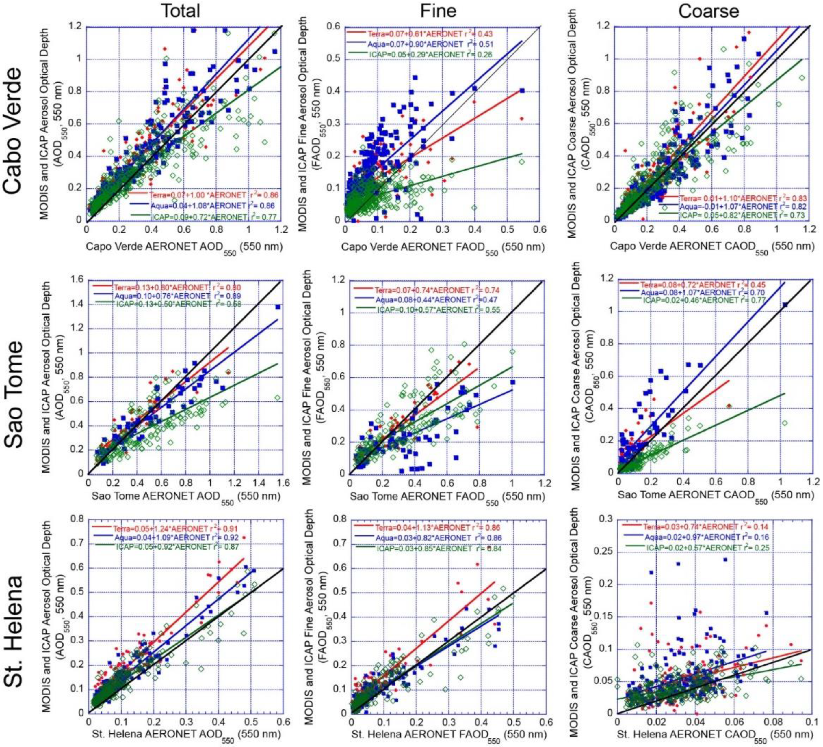
4.1. Littoral Example: African Land Plumes

From Section 3.1, there are numerous regions of notable correlated error, with particularly strong biases between products in the littoral regions and terrestrial air masses that are transported over the oceans. For remote sensing, these regions host the highest maritime AODs and the best signal-to-noise ratios. At the same time, the littoral regions are a challenge for models as they must cope with the littoral transition in meteorology while having inherently different skills in satellite products and data assimilation between land and ocean. Based on Figure 4, some of the strongest areas of bias between products are littoral Atlantic–Africa, which is also associated with a change in particle speciation: a dust-dominated Saharan dust plume (30°−15°N; 15°−35°W) centered around Cabo Verde, which transitions into mixed dust, biomass burning, and pollution sector, into a Sahel/Gulf of Guinea sector (~15°N to the equator; 25°W to 1°E), and eventually into biomass burning dominated central Africa (~equator to 15°S; 5°W−15°E). This variability in loading and speciation makes Africa an ideal natural laboratory for identifying errors associated with specific sources and more extreme events. Scatter plots of all available data from Terra and Aqua MODIS and the C4C for these three regions are provided in Figure 13 with tabular data in Table 5. While we are concerned about island effects, to investigate consistency and increase the overall dataset throughout the year, AERONET sites are also available for an SDA style analysis in each of the domains: Cabo Verde, Sao Tome, and St. Helena, respectively (Table 6; Figure 14). These were processed identically, with the exception of a daily averaging temporal window. In all cases, the nature of magnitude-dependent errors of MODIS and the C4C is such that there is typically a positive ordinate/y intercept that is then compensated for by slope. Therefore, one should also examine data in the context of the black 1:1 line provided. Inspection of Figure 13 shows that serendipitously there is a natural break in AOD550 at the 0.28/84th percentile level.
As in the global analysis, all MAN data points have an associated C4C product. For MODIS, sampling is greatly reduced. Even with a +/−2 h window, the resulting yield was <1/3. Nevertheless, findings are largely consistent with the global analysis, especially given that the high AOD550 events are largely from this domain. Due to Africa hosting the largest dust and biomass burning sources in the world, AOD550 signals from MAN are high. The mean AOD550 values for Cabo Verde, the Sahel/Gulf of Guinea, and central African subsets were 0.23 ± 0.19, 0.37 ± 0.26, and 0.29 ± 0.16. Given how few samples are available (545, 534, 102, again, respectively), these should not be taken as climatological values but rather as a marker of error relative to the median value of AOD550 of 0.08 in the entire dataset. MODIS scores particularly well, generally better than the published error budget of 0.05 + 0.15 × AOD550 [29]. C4C errors are generally on par with MODIS for AOD550 < 0.28, but with enhanced scatter for values between 0.4 and 0.8 and a distinct low bias for the only four data points available thereafter. Much of this scatter attributed to outliers is generated as a result of individual model outliers within the consensus. Errors of the fine/coarse partition are also largely consistent with the global findings—not surprising that the Atlantic–African domain contributes significantly to the population of higher AOD.

4.1.1. Cabo Verde as an Indicator of a Dust Dominated Regime

Cabo Verde dust-dominated domain demonstrates the highest magnitude bias in FAOD550 between satellite and models. As expected for a region dominated by Saharan dust, the MAN fine mode fraction is ~0.32 up to the 84th AOD550 percentile, reducing further to 0.21 thereafter. Total AOD550 correlations and errors are generally good. However, MODIS clearly biases high for FAOD550 and η550 in this dust-dominated regime. Aqua MODIS also has a slight AOD550 and CAOD550 high bias as well. The AERONET site at Cabo Verde can also provide 364 level 2 data points between 3 January 2016 and 9 December 2018 to the analysis, giving results similar to MAN. These data suggest the regional features in Figure 3 are a result of overall AOD550 and CAOD550 low bias in the C4C and a slight high bias in MODIS counterparts. Further, while there is significant scatter (particularly in Terra MODIS), part of the overall MODIS AOD550 is due to enhanced FAOD550 attribution.
Given how significant the AODs can be for dust transported from the Sahara, even small errors in fine mode fraction can result in significant FAOD errors relative to the global ocean baseline. The MODIS FAOD550 bias can possibly be attributed to either the optical model and/or definitional issues. The use of the SDA for MAN and AERONET is consistent with evaluating the two-mode optical model used in the MODIS retrieval. Thus, the best available evidence is that perhaps the MODIS retrieval requires further tuning. Such tuning would likewise resolve the difference with the C4C. This said, as noted in Section 2, the differing model definitions of fine and coarse mode aerosols can and do lead to ambiguities in the fine mode fraction. Ongoing studies show that the use of the AERONETs DK retrieved FMF and FAOD550 would resolve some of the FAOD550 bias, with further ambiguity in the issue of the particle size distribution minimum and the restricted set of retrieved diameters that define it. This would then result in a higher CAOD550 bias, with AOD550, of course, remaining unchanged.
Regarding the C4C performance, it is noteworthy that there are several FAOD550 populations. First, for the lowest FAODs, the C4C has a clear high bias. As noted in the global analysis, this is persistent. Currently, developers are investigating the nature of this background FAOD550, but it is likely due to a combination of interacting factors: sources, transport, over diffusion and/or numerical diffusion, and data assimilation. For higher MAN and AERONET FAOD550, there is a bifurcation of C4C performance, with periods when FAOD550 is reasonably well captured and those when it is missed. The underrepresented FAOD550 cases are all associated with lower η550 and higher AOD550. The explanation is two-fold. In this case, there are also definitional issues. Within the C4C, all dust in each of the models is assigned to the coarse mode when in fact, three of the four models have explicit fine mode dust bins. Normally, this results in small errors, but in the case of large dust events, it does result in a detectible bias in absolute magnitude, even if it is a small fractional error in the AOD budget. Second, this bias is then compounded by the overall low bias in high AOD550 events.

4.1.2. Sahel and Gulf of Guinea as an Indicator of a Mixed Environment

The Sahel/Gulf of Guinea region was also well sampled by MAN (536 obs.) and measured the highest average AOD550 of all of the sub-regions discussed in Section 4 (mean and standard deviation 0.37 ± 0.26). The region is a receptor for many sources, with MAN sampled η550 =0.43 and 0.33 for AOD550 less than and greater than 0.28. The C4C attributes ~50% of total AOD550 to dust, ~25% to the Sahel and tropical African biomass burning, ~15% to pollution/sulfate-based species, and ~10% to background sea salt. Despite this diversity in the region’s sources, MODIS and the C4C score well between each other and MAN. For AOD up to and a little beyond 0.28, all products score well across components. For higher AOD550, the C4C again exhibits its low bias for AOD550 and CAOD550. While it is not readily apparent in Figure 13, when the data are examined in bulk (Table 5), the fine mode in Terra and Aqua are still slightly high biased relative to the coarse mode.
There are no offshore AERONET sites that are located in the middle of this domain, but the Sao Tome site is located at the southern boundary, on the equator, and 300 km offshore of mainland Africa. However, from an aerosol characteristics point of view, it is closer to the Gulf of Guinea domain than central Africa. The Sao Tome site provided an additional 153 daily average samples for the analysis. Overall, the results are very similar to the MAN domains but with a slight reduction in skill as the environment transitions from the Gulf of Guinea to the central African domain. A bifurcation of C4C data above and below the 1:1 line is noticeable for both AOD550 and FAOD550. This is largely seasonal, with the C4C over-predicting these quantities in the late fall to early spring and under-predicting during the core June–October biomass burning season. Terra and Aqua MODIS continue to show good skill on AOD550, but they too show more uncertainty in the fine/coarse partition. These are not related to the annual cycle. Oddly, Aqua MODIS, which has the highest skill on AOD550, has the lowest for FAOD550.
The Gulf of Guinea demonstrates that even in complex environments, Earth systems tools have good skills. MODIS, in some ways, may represent a “Goldilocks zone” case, where signals are high and with middling fine/coarse where partitioning errors can go either way. MODIS skill is nevertheless impressive for the available datasets. Interestingly, the C4C has improved bulk errors and regression over MODIS for the MAN dataset, demonstrating that Earth system models have considerable skills, perhaps for some of the same reasons. For this region, data assimilation in models may also result in significant benefits. In this region, the land surface transitions from desert to cropland to tropical, and with it, to a less challenging lower boundary condition.

4.1.3. Central Africa and Biomass Burning

Compared to the Cabo Verde and Gulf of Guinea regions, there are many fewer MAN data points available (102). These were collected over several years in December through March, when AOD550 are generally lower, and in October 2016 from one cruise as the biomass burning season was waning. Thus, MAN did not capture the peak burning season during our study period nor can it resolve the impact of the region’s well-defined seasonal cycle in biomass burning single scattering albedo on MODIS error [76]. Total MAN AOD550 was nevertheless impressive, with mean and standard deviation values of 0.29 ± 0.16. However, with a mean and median η550 of 0.63 and 0.75, this particular data population is still largely mixed. Overall, the C4C suggests average AOD550 fractions of 10% dust, 15% sea salt, 50% biomass burning, and 25% sulfate-based pollution. Observation numbers are almost evenly split at the AOD550 of 0.28 with two modes of lower and higher AOD550 conditions (means of 0.13 and 0.42 for each category). From Figure 2 and Figure 3, the central African smoke plume presents a strong AOD550 feature, which compares reasonably well between Aqua MODIS and the C4C, with some AOD dependence. Relative to Aqua MODIS, the C4C is overestimating FAOD550 and η550 and underestimating CAOD550. Against Terra, the signs of the bias in the C4C remain the same, although lesser in magnitude. Aqua also shows a population of low biased FAOD550 points. However, one must also consider there are only eight Terra observations available. The central Africa feature also hosts some of the strongest biases in the fine/coarse partition. The C4C has the largest overall biases, with the C4C over-predicting FAOD550 and η550. At the same time, MODIS Aqua also has biases almost as significant but opposite in sign. This results in a large difference between the two in Figure 3. Here is a situation opposite to Cabo Verde in η550 but for the fine dominated environments, underrepresenting the residual coarse mode.
Given how few MAN samples there are and that they miss the peak burning season, the Saint Helena AERONET site can help to fill in the dataset. However, at 1900 km offshore of Africa, and in an overall unbiased region between MODIS and the C4C, it should really be labeled a marine receptor rather than littoral. Despite being 1/3 of the distance to South America, African biomass burning strongly modulates both AOD550 and FAOD550. Overall correlations are excellent for these parameters, but with a consistent high bias for all parameters in this case for low AOD550 values. The C4C is slightly less biased than MODIS. At such a distance from shore, there would be multiple opportunities for data assimilation. One interesting aspect of the site, however, is related to coarse mode. Unlike other regions, all products are biased high, and the MODIS products have numerous significant outliers. These are not related to cloud fraction or mixing state and occur at all times of the year. These CAOD550 outliers do, however, tend to be associated with higher AOD550 biases. In order to help resolve this error, a hand analysis was performed. Outliers were associated with a host of marine boundary layer cloud types and morphologies (clear with near subpixel small cumulus to holes in stratiform). Further, the MODIS AOD550 fields did not show high variability but showed low variance from retrieval to retrieval (~0.02). This could be due to coastal effects on coarse mode lifecycle near the AERONET site or a variety of cloud artifacts in MODIS DT.

4.2. Latidudinal Dependencies of Remote Maritime Environments

The differences between products in the remote maritime environment are perhaps the most difficult to fully evaluate but, at the same time, may be the most important to understand to estimate indirect aerosol forcing. Compared to the littoral, aerosol loadings are low, and there are few verification observations, especially for higher wind conditions. Small biases can lead to significant interpretation differences. Data were segregated into three domains that exhibited bias from Figure 3: (1) Southern Oceans (Latitude < 30°S), where the C4C under and over-predicts FAOD550 and CAOD550, respectively, relative to Aqua MODIS. This also results in a low bias in η550 in the C4C over Aqua MODIS. (2) The subtropical and tropical Pacific Basin (30°S−30°N), where the C4C is under-predicting AOD550, FAOD550, and CAOD550 relative to Aqua MODIS. Lastly, (3) 30° to 60°N, where Aqua MODIS and the C4C generally match but with slight local perturbations. Scatter plots for these regimes are provided in Figure 15, with corresponding data in Table 7. In order to improve visibility in some of the scatter plots, some extreme data points are off-scale (<3 per plot) but are included in Table 7 statistics. As mentioned, the number of AERONET sites operating in remote ocean locations is dwindling. Those that do exist are often located on the leeward side of the islands. There are three sites, however, that have some verification potential in their remoteness and location relative to the island that was reported during our study period: (1) Macquarie Island, south of New Zealand (54.5°S; 158.8°E); (2) Kwajalein Atoll in the tropical Pacific (8.8°N; 167.7°E); (3) Graciosa Island in the Azores (39.1°N; 28.0°W). These are included in Figure 16 and Table 8.

4.2.1. Southern Oceans

The southern oceans region spans the sub-tropics to the Antarctic, and hence a variety of truly maritime conditions. The Southern Ocean’s “roaring 40’s” high winds and high cloud fraction epitomize extreme maritime weather, and here is where there are the most significant deviations in FAOD550 and CAOD550 between MODIS and the C4C (e.g., Figure 4). Given the remoteness of the Southern Oceans domain, there was a respectable 1384 hourly MAN observations available. However, the median, mean, and standard deviation of all MAN AOD550 samples were a mere 0.03, 0.04, and ±0.03, with a maximum of 0.23. That is, the median AOD is at the single sample noise floor for SDA. Likewise, mean FAOD550 and CAOD550 were derived from the SDA average of 0.015 and 0.025 respectively (below what we would consider the noise floor), with corresponding maximum values of 0.17 and 0.20. Based on the C4C speciation, perturbations in the CAOD550 above 0.04 are almost entirely described as sea salt with occasional residual <0.01–0.02 dust, perhaps from Patagonia [77]. As noted in Section 2, the fine mode source specification for the sample set is ambiguous but largely associated with the ICAP sulfate-dominated “anthropogenic/biogenic fine” over more occasional organic “biomass burning categories” originating from Africa, Australia, and South America. Based on the SDA values, for typical conditions, MAN’s η550 is 0.43 (slightly coarse dominated), with a more dominant coarse mode for higher AOD550 values such as above 0.08 when we expect SDA to be clear of noise issues (MAN η550 values of 0.34 to 0.26).
The MAN values demonstrate how pristine the southern oceans can be, the dominance of coarse sea salt there, and the small margins in AOD the community is facing. Nevertheless, as observed in Figure 4, Aqua MODIS and the C4C both have similar values in AOD550 for the southern oceans on the order of 0.12 to 0.18, significantly higher than the MAN mean. This indicated a sample bias in MAN; not surprising given how few austral winter observations are made. Indeed, the latitude band of the highest AODs, 45°–60°S, has only 100 MAN observations, and these we suspect are for fair weather. For this sample, both MODIS and the C4C are slightly high-biased relative to MAN observations for observations up to 0.12 manifest in the fine mode. This environment, and the lack of observations, challenge the community.
Because the observed AOD550 value is so close to zero, and the definite positive nature of the models and proclivity to MODIS retrieval tuning to prevent negative retrievals, these products almost have to be highly biased in AOD550. However, there is consistency in findings with higher AOD550 where SDA is well above the noise floor, as well as with the global analysis. Even if the MAN SDA calculations are discounted, the AOD550 biases stand, and the differences in the southern oceans between MODIS and the C4C is a mere 0.01–0.02 difference in their calculated FAOD550. While the bulk error statistics for the southern oceans are impressive (if sample biased), from examining the scatter plots in Figure 15, it is clear that while overall the error distributions are low, there are areas of AOD550 over-reporting in MODIS and the C4C. Positive biases for FAOD550 and CAOD550 are particularly large for high and low AOD550, respectively. While one can question the efficacy of SDA for such low AODs, these deviations for total AOD550 are significant in absolute terms-well above the MAN noise floor. SDA is suggestive of populations of high bias in MODIS and the C4C alike. The collective circumstantial evidence again points to an overestimate of the fine mode.
The AERONET site that is part of the Atmospheric Radiation Measurement (ARM) program mobile facility deployment to Macquarie Island, south of New Zealand, provides what is perhaps a less sample-biased dataset for the southern oceans. The site was located on the northern tip of the island (54.5°S; 158.9°E) without any obstruction to the East–Northeast to South–Southwest sides, providing better exposure to the windward side of the ocean than any other site in this regime. This said, there was a 200 m hill terminating immediately to the windward side, likely inducing some terrain effects. The site successfully generated data for nearly 2 years (20 April 2016 to 12 March 2018). A total of 97 daily average measurements were made with AOD550 (0.075 ± 0.028), significantly higher and with more spread than the MAN counterparts. Results for bias and RMSD in AOD550 deviated somewhat from MAN. While the overall tendencies remain for all systems being high biased in AOD550 and FAOD550 for this dataset, it is the C4C that has higher biases than both MODIS. For C4C consensus members, there are some cases of extreme bias in FAOD550. These were linked to specific models that appear to be overproducing fine mode particles in secondary production. Likewise, one unrelated model to this bias model stands out for a high coarse mode. Combined, it is likely that the C4C and MODIS are overestimating AODs and their components in this region.

4.2.2. Tropical and Subtropical Pacific

For the subtropical and tropical Pacific, 727 MAN observations were made. Aerosol loadings are higher, span greater magnitudes, and appear to be better behaved than their southern hemisphere counterparts. Mean, median and standard deviations in MAN observed AOD550 (0.085, 0.075, and ±0.045, respectively) are not dramatically dissimilar to the C4C and MODIS, suggesting less MAN sample bias. η550 for this region is also higher than the southern oceans (η550 = 0.35–0.45), indicative of an even greater influence of additional terrestrial transport events. Notable in Figure 15 and Table 7 is that, similar to the global analysis, there is a fairly consistent positive offset in all products for AOD550. Likewise, FAOD550 behaves somewhat similarly to the southern oceans, with higher FAOD550 biases and, in particular, a small population of significant positive outliers in the satellite data. For the C4C, a noticeable difference in this maritime region exists for the coarse mode. Here the C4C products have a distinct low bias in CAOD550, which could be due to a combination of (1) underproduction (as was aforementioned hypothesized), (2) aggressive wet scavenging (not uncommon in models in these kinds of environments [78], and/or (3) underestimation of the coarse mode hygroscopicity within a global model.
The best AERONET counterpart for the tropical and subtropical Pacific regime is the Kwajalein Atoll site, located on the edge of the atoll, which has a maximum elevation of 10 m. With consistent easterly trade winds, the site is one of the most remote AERONET sites and is far from terrestrial sources. This site provided 85 daily averaged data points and roughly one year of level 1.5 data from 26 October 2018 to 3 December 2019. For such a remote location, both MODIS and the C4C have excellent correlations but typical high biases in AOD550 and FAOD550 (Figure 15). The C4C correlates better and is less biased than MODIS, largely due to significant positive biases in MODIS FAOD550. As the average MODIS cloud fraction is 70% for this site, the FAOD550 high bias in both instruments is consistent with the MAN-based cloud fraction analysis in Section 3.4.1. Overall, at this remote location, variability in AOD is related to the coarse mode rather than fine, which scores particularly well for all systems, especially the C4C. This is different from MAN, which suggested an overall coarse mode with low bias. One other noteworthy aspect of the dataset is that there were occasional fine mode enhancements that were well captured by the C4C and can be viewed as a separate population in both MODIS instruments. While they cannot be currently sourced, model output is consistent with long-range residual transport from East Asia by the westerlies that somehow worked their way into the easterly trades. These cases are consistent with the long-range transport of terrestrial sources modulating remote CCN budgets.
However, overall, it is clear that the global findings are applicable to the remote tropical to subtropical Pacific, and fine mode aerosol species are overestimated. While MAN suggests that the coarse mode sea salt production is either under-produced or over-scavenged, the Kwajalein site shows outstanding performance. More work is clearly necessary to resolve these differences.

4.2.3. Northern Mid Latitudes

Of the three core maritime regions, the northern mid-latitudes have the highest MAN AOD550 values and spread (AOD550 mean = 0.10, median = 0.08, standard deviation = ±0.09). Thus while the mid-latitudes show the best-behaved regressions of the three large domains, bulk error statistics are largely comparable to the other domains. This region hosts significant terrestrial transport, and thus has the highest FAOD550 η550 values (mean FAOD550 = 0.06; η550 = 0.54). Biases as a function of AOD550 are on par with the other regions (i.e., high biased AOD550, FAOD550). One notable point is the C4C low bias in CAOD550 has largely recovered from the tropical/subtropical Pacific. This implies a latitudinal bias in the C4C coarse mode from good but overestimated skill in the southern oceans, to a low to a neutral bias in the tropics to subtropics, then to reasonably good overall skill in the northern mid-latitude oceans.
There are few good options for AERONET comparisons in this regime, with nearly all associated with significant land masses. The one potential site is Graciosa Island, Azores, where AERONET was deployed as part of the ARM mobile facility with data reporting from 1 January 2016 to 24 June 2019. Four hundred and fifty-two daily average data points were generated, the largest of the AERONET sites examined in this paper. The C4C suggests this site is largely impacted by long-range transport of sulfate-based pollution and sea salt, though occasional intrusions of African dust and organic/biomass burning occur. Findings are consistent with MAN and the overall analysis, including an overall good skill but with high biases in AOD and FAOD550. Similar to the Kwajalein site, the high bias by both MODIS instruments in FAOD550 is particularly visible.

5. Conclusions

Most of the globe can be categorized as a remote maritime environment where the sensitivity of clouds to CCN perturbations is expected to be high. Despite the complexity of closing the CCN budget, climate scientists have to resort to simple metrics such as total, fine, and coarse AOD550 to monitor aerosol events globally, using satellites as well as models in which satellite data are assimilated. This study is the first of several steps in joint remote sensing and modeling error analysis in which remote sensing-based MODIS MOD/MYD 04 Dark Target and model-based ICAP-MME Core Four Consensus (C4C, average of CAMS, GEOS, MASINGAR, and NAAPS) optical depth products are compared, with differences adjudicated against the shipboard MAN sun photometer network. The MODIS Dark Target represents the most widely used aerosol remote sensing product, and C4C was shown to provide the best available operational model analysis guidance for monitoring global AOD fields. Despite the evaluation and shortcomings found here, overall, we found both MODIS DT and the C4C performed admirably. However, persistent and spatially correlated biases, if not corrected, likely result in significant uncertainty if used in high fidelity applications, such as inverse modeling.
As the first step in this study, bulk comparisons were performed in Section 3.1 between Aqua MODIS and the C4C in order to identify regions of correlated bias in AOD550, FAOD550, CAOD550, and η550 that require further investigation. This comparison showed:
(1)
Because the contributing C4C models assimilate MODIS AOD550, Aqua MODIS and the C4C generally compare well to each other in their AOD550 fields in the maritime environment. However, areas of correlated bias were identified, even for pairwise samples. Areas of spatial bias were found to be even more pronounced in a fine versus coarse AOD550. Since the contributing C4C models assimilate only total AOD550 and not products related to aerosol size (Ångström Exponent, FAOD550, or CAOD550), the contribution of individual aerosol species to total AOD550 and the partitioning to fine and coarse aerosol modes depends on the parameterizations within each respective model;
(2)
The most prominent areas of spatially correlated bias in the maritime environment between MODIS DT and the C4C are near terrestrial source regions. MODIS DT has notably higher AOD550 and FAOD550 than the C4C for the Saharan dust plume but lower FAOD550 for Central Africa biomass burning advection. For CAOD550, MODIS has much higher values than the C4C offshore of the Sahel, Gulf of Guinea, and Arabian Gulf regions;
(3)
For more remote marine environments, there is a small but persistent latitudinal difference between MODIS and the C4C. MODIS generates higher AODs over the tropics to subtropics (up to 0.03 relative to a 0.15 baseline), as well as in the Arctic and Antarctic. The C4C, on the other hand, provides slightly higher AOD550 and CAOD550 in the mid-latitudes. In nearly all latitudes, the MODIS retrieval provides higher FAOD550 and η550 than the models. Some sources of disagreement are obvious, like the C4C underestimating the transport of high AOD events from boreal biomass burning to the sub-arctic and arctic. Over most of the remote oceans, the cause of the observed differences is not immediately clear.
In order to help explain the findings outlined above, Terra and Aqua MODIS and the C4C were compared to 8637 independent MAN data points collected over the globe in Section 3.2. In summary:
(1)
While correlations of MODIS to MAN are very good, Aqua MODIS retrievals have slight but persistent diagnostic high biases in AOD ranging from + 0.02 to +0.04, and RMSDs of 0.02–0.05 for AOD550 < 0.28. Terra MODIS has even higher values in bias and RMSD by an additional +0.01 above Aqua. These biases and performances have long been known in the community. However, the presented analysis indicates that the biases are likely associated with a systematically high biased η550 and FAOD550 rather than CAOD550 in the retrieval. This is consistent with brief reports in the literature of potentially high bias in retrieved Ångström Exponent in the MODIS maritime AOD product [29]. Therefore, the community should consider MODIS DT AOD550, FAOD550, and η550 as high biased;
(2)
The C4C also showed a good correlation with MAN and showed similar but slightly lower biases and RMSDs as its MODIS counterparts for AOD550 < 0.28. The C4C is also highly biased in η550 and FAOD550 rather than CAOD550, even though the models only assimilate total AOD550. As a consensus, the C4C provided better global performance than any individual model, and all four C4C members have similar signs of bias in each region. Therefore, the community should also consider the C4C AODs, FAOD550, and η550 as high biased for AOD550 < 0.28. The slightly better skill in the models over the fundamental MODIS retrieval for a global dataset is understandable given that all data assimilation systems quality assure and, to some degree, bias correct retrieved AOD550 values before assimilation;
(3)
As AOD550 increases from 0.28 to over 1, the MODIS retrievals begin to outperform the C4C in both bias and RMSD. In general, MODIS is still positively biased in AOD550 and FAOD550. Whereas Aqua MODIS remains unbiased in the coarse mode with increasing AOD550, MODIS Terra becomes further biased in CAOD550. In contrast, the C4C has a distinct low bias that is consistent with previously published analyses of the C4C against AERONET [30];
(4)
Both pairwise and prognostic error analyses were performed, including those data points that intersect with both Terra and Aqua MODIS, and the results indicate that the study findings do not appear to be sample biased in regard to the total number of samples. Further, by examining prognostic versus diagnostic error, it was found that when a lower AOD or η550 value is retrieved by MODIS or predicted by the C4C, it is more likely to be near that value. Nevertheless, the signs of the biases largely remain for prognostic versus diagnostic error. Finally, the estimated clear-sky bias of the overall MODIS dataset (estimated by taking the ratio of C4C data with corresponding MODIS Aqua data to all data) is similar to other studies [15] with the clear sky maritime environment having lower AODs on the order of 10–20%. The exception to this is the North Atlantic, where clear sky conditions have higher AOD550, likely due to biomass burning.
An analysis was performed to assess the relationships between bias to cloud mask fraction and surface wind speed. From this analysis, it is concluded that:
(1)
While the complete MODIS DT dataset has only a small overall clear sky sampling bias, verification with MAN shows a well correlated and increasing positive bias with increasing cloud fraction. The Aqua MODIS bias at 80% cloud fraction reaches levels of +0.05, +0.04, and +0.01 for AOD550, FAOD550, and CAOD550, respectively, and explains significant positive outliers for lower MAN AODs. Terra MODIS showed similar results with a +0.01 further bias added to AOD550 and FAOD550. Therefore, positive error in MODIS DT AOD550 retrievals due to the presence of clouds manifests itself with the retrieved fine mode, not the coarse mode, as one would expect for the addition of spectrally flat radiances from, say, an under-restrictive cloud mask. While it is believed that 3D radiation effects and cloud detrainment may contribute, the bias is constant as a function of background AOD550. Thus, the suspected issue remains with the MODIS cloud mask and how the retrieval parses radiances to its fine and coarse modes. A second possibility is that Rayleigh scattering contributions need to be updated to account for 3D effects. It should be noted that given the probability of a MAN observation is increased for low cloud fractions, but global maritime cloud fractions are high, MODIS errors diagnosed in this study are likely underestimated, perhaps by 50% or more;
(2)
The C4C also shows some very slight +/−0.01 positive and negative cloud fraction dependency with FAOD550 and CAOD550 respectively, connected to 80 and 90% cloud fractions. This may be related to meteorological conditions associated with high cloud cover;
(3)
For winds less than 12 m s−1, both MODIS DT and the C4C generally have constant biases in AOD550 components. For higher wind speed, MODIS instruments develop a more positive FAOD550 bias, perhaps due to the lower boundary condition or further confusion of coarse mode for the fine mode. The C4C has a very slight −0.01 bias in CAOD550 for wind speeds less than 12 m s−1, changing signs to a positive bias in CAOD550 in the consensus and in all members for wind speeds beyond this point (although one member has a notably stronger bias than the others). This suggests that the C4C models are overproducing sea salt and hence CAOD550 for the mid-latitude oceans. This is especially true for the southern oceans, where the CAOD550 bias may be as much as +0.04.
While the findings presented above were drawn for the entirety of the MAN-product matched dataset, the bulk comparisons in Section 3.1 showed noticeable areas of correlated bias, including land plumes of terrestrial aerosol origin as well as a latitudinal dependence in bias. As a result, the generalized findings above were scrutinized for specific maritime regions that also hosted an appropriate AERONET site.
(1)
In order to investigate terrestrial aerosol-related sources, three areas of the Atlantic associated with African land plumes were examined in detail, including the Cape Verde region for dust, the Sahel/Gulf of Guinea for aerosol mixtures, and Central Africa for biomass burning. (i) For the Saharan plume, all products do well for dust, although the C4C does indeed under-predict significant events. In regards to the differences in FAOD550 and η550, the evaluation indicates that MODIS does assign a slightly higher FAOD550 and η550 than the C4C for dust, further compounded by the high AOD550 for significant events. Further investigation is needed to assess if MODIS DT optical models need to be adjusted to reduce the fine mode fraction for dust. (ii) In the mixed aerosol environments of the Gulf of Guinea, all products perform admirably but with biases consistent in the global analysis. (iii) For Central Africa, there is a slight positive bias in AOD and FAOD550 in all products. However, the C4C struggles with the coarse mode in the littoral regions just offshore, perhaps due to unresolved mesoscale phenomena. Based on an examination of the St. Helena site, which is located far offshore, the C4C recovers skill in CAOD550, and it is MODIS that demonstrates occasional positive outliers;
(2)
The second set of in-depth studies was performed to investigate the latitudinal differences between MODIS and the C4C. (i) In the southern oceans (<30°S), C4C models only slightly overproduce the coarse mode against MAN. For the fine mode, there are significant outliers for MODIS and some C4C members. However, MAN data appears to be sample-biased towards calmer conditions and the edges of the high wind region, with very pristine conditions being sampled. Compared to Macquarie Island AERONET site within the southern ocean high wind belt, MODIS AODs, errors, and biases are slightly bigger. The C4C and its members have higher biases than MODIS DT in all components. This appears to be associated with both sea salt and secondary overproduction. (ii) For the tropics to subtropics (30°S−30°N), MODIS DT and the C4C performed reasonably well against MAN but with clear high biases in AOD550 and FAOD550, including significant outliers in MODIS DT FAOD550, presumably due to cloud mask shortcomings. At the Kwajalein Atoll AERONET site, one of the most remote within the network, MODIS has good skill in AOD550 and CAOD550 yet appears to be highly biased in FAOD550 with virtually no skill. Further, at Kwajalein, the C4C clearly outperformed MODIS DT. MODIS deficiencies appear to be associated with cloud-related biases as well as, perhaps, the aerosol optical models. (iii) Finally, for the northern mid-latitudes, we examined the 30°N to 60°N dataset, along with the Graciosa Island, Azores AERONET site. Overall, both MODIS and the C4C showed the best skill in AOD550 of any remote maritime region investigated for most parameters. However, high biases in AOD550 and FAOD550 were persistent. For unknown reasons, unlike Aqua, Terra MODIS has virtually no skill in CAOD550 at the Graciosa Island AERONET site.
Finally, regional or conditional biases between the MODIS and C4C products described above are informative to the community’s skill, and challenges in monitoring aerosol lifecycle. The results of this analysis indicate that attention is required for the further resolution of fine versus coarse partitioning of AOD550 in both definition and method. Given how small the aerosol signal is over most of the oceans, the relatively low biases presented here should perhaps be seen as a positive for the community. Nevertheless, as the community moves towards more sophisticated analyses, spatially correlated biases can dramatically influence our interpretation of key aerosol and cloud processes-especially for inverse studies. MODIS DT is preferable to models for investigating individual events but has challenges due to cloud-related issues, either with the cloud mask or perhaps 3D RT effects. Some attention is also required on the optical models attributing AOD550 to its fine and coarse mode components. In regards to aerosol operational models and their reanalysis counterparts, these products merge models with remote sensing through data assimilation and are probably more useful and user-friendly for many climate studies. They underwent significant development and, as a result, are increasingly used. For most cases, the C4C has lower bias and RMSD than MODIS DT for most of the world’s oceans, but biases nevertheless have remnant correlations with MODIS, and the under-prediction of significant events remains a problem. Both model bias and event shortcomings are rooted in the model dependencies on the process that are complex and have errors that integrate with time, with occasional updates from an observable as blunt as AOD550. Nevertheless, the models performed admirably, and further improvements are expected in the coming years. The most significant areas of attention for the open ocean include sea salt production/scavenging and secondary aerosol production, to remove biases in the models. The transition from terrestrial sources to the maritime environment, both in terms of global source functions and meteorology, will require attention along a broad front.

Author Contributions

Conceptualization, J.S.R.; methodology, J.S.R., A.G., J.Z., R.E.H., A.S. and N.T.O.; software, A.G. and J.Z.; validation, J.S.R., J.Z., A.S., T.F.E. and R.C.L.; formal analysis, J.S.R.; investigation, J.S.R., N.T.O., P.X., R.C.L., A.S. and T.F.E.; resources, J.S.R. and P.X.; data curation, A.G., A.S., T.F.E., J.Z., E.A.R., P.R.C., P.X., A.B. and T.T.; writing—original draft preparation, J.S.R., R.E.H., J.I.R., N.T.O. and R.C.L.; writing—review and editing, J.S.R., E.A.R. and J.I.R.; visualization, A.G.; supervision, J.S.R. and R.E.H.; project administration, J.S.R. and R.E.H.; funding, J.S.R. and R.E.H. All authors have read and agreed to the published version of the manuscript.

Funding

Funding for this project was across multiple agencies to support data generation, synthesis and analysis. This analysis and composition for this research was funded by was provided by the US Naval Research Laboratory Base Program, the Office of Naval Research, and NASA.

Data Availability Statement

Data for this study is available from the following sources, all last accessed on 7 June 2022: MODIS data is available at the NASA Goddard Space Flight Center Level-1 and Atmosphere Archive and Distribution System (LAADS; https://ladsweb.modaps.eosdis.nasa.gov/); MAN and AERONET data used in this study can be found at https://aeronet.gsfc.nasa.gov/; and ICAP consensus products archived at https://usgodae.org.

Acknowledgments

We gratefully acknowledge the many investigators that support the federated Marine Aerosol and Aerosol Robotic Networks. We are likewise grateful to the many investigators and support staff that keep operational aerosol models operating.

Conflicts of Interest

The authors declare no conflict of interest.

References

  1. Charlson, R.; Lovelock, J.; Andreae, M.; Warren, S. Oceanic phytoplankton, atmospheric sulphur, cloud albedo and climate. Nature 1987, 326, 655. [Google Scholar] [CrossRef]
  2. Clarke, A.D.; Ki, Z.; Litchy, M. Aerosol dynamics in the equatorial Pacific marine boundary layer: Microphysics, diurnal cycles and entrainment. Geophys. Res. Lett. 1996, 23, 733–736. [Google Scholar] [CrossRef]
  3. Clarke, A.D.; Freitag, S.; Simpson, R.M.C.; Hudson, J.G.; Howell, S.G.; Brekhovskikh, V.L.; Campos, T.; Kapustin, V.N.; Zhou, J. Free troposphere as a major source of CCN for the equatorial pacific boundary layer: Long-range transport and teleconnections. Atmos. Chem. Phys. 2013, 13, 7511–7529. [Google Scholar] [CrossRef] [Green Version]
  4. Mechoso, C.R.; Wood, R.; Weller, R.; Bretherton, C.S.; Clarke, A.D.; Coe, H.; Fairall, C.; Farrar, J.T.; Feingold, G.; Garreaud, R.; et al. Ocean–Cloud–Atmosphere–Land Interactions in the Southeastern Pacific: The VOCALS Program. Bull. Am. Meteorol. Soc. 2014, 95, 357–375. [Google Scholar] [CrossRef] [Green Version]
  5. Quinn, P.; Coffman, D.; Johnson, J.; Upchurch, L.M.; Bates, T.S. Small fraction of marine cloud condensation nuclei made up of sea spray aerosol. Nat. Geosci. 2017, 10, 674–679. [Google Scholar] [CrossRef]
  6. Twohy, C.H.; DeMott, P.J.; Russell, L.M.; Toohey, D.W.; Rainwater, B.; Geiss, R.; Sanchez, K.J.; Lewis, S.; Roberts, G.C.; Humphries, R.S.; et al. Cloud-nucleating particles over the Southern Ocean in a changing climate. Earth’s Future 2021, 9, e2020EF001673. [Google Scholar] [CrossRef]
  7. Ayers, G.P.; Cainey, J.M. The CLAW hypothesis: A review of the major developments. Environ. Chem. 2007, 4, 366–374. [Google Scholar] [CrossRef]
  8. Carslaw, K.S.; Boucher, O.; Spracklen, D.V.; Mann, G.W.; Rae, J.G.L.; Woodward, S.; Kulmala, M. A review of natural aerosol interactions and feedbacks within the Earth system. Atmos. Chem. Phys. 2010, 10, 1701–1737. [Google Scholar] [CrossRef] [Green Version]
  9. Behrenfeld, M.J.; Moore, R.H.; Hostetler, C.A.; Graff, J.; Gaube, P.; Russell, L.M.; Chen, G.; Doney, S.C.; Giovannoni, S.; Liu, H.; et al. The North Atlantic Aerosol and Marine Ecosystem Study (NAAMES), Science Motive and Mission Overview. Front. Mar. Sci. 2019, 6, 122. [Google Scholar] [CrossRef]
  10. Regayre, L.A.; Schmale, J.; Johnson, J.S.; Tatzelt, C.; Baccarini, A.; Henning, S.; Yoshioka, M.; Stratmann, F.; Gysel-Beer, M.; Grosvenor, D.P.; et al. The value of remote marine aerosol measurements for constraining radiative forcing uncertainty. Atmos. Chem. Phys. 2020, 20, 10063–10072. [Google Scholar] [CrossRef]
  11. Spencer, R.S.; Levy, R.C.; Remer, L.A.; Mattoo, S.; Hlavka, D.; Arnold, G.; Platnick, S.; Marshak, A.; Wilcox, E. Exploring aerosols near clouds with high-spatial-resolution aircraft remote sensing during SEAC4RS. J. Geophys. Res. 2019, 124, 2148–2173. [Google Scholar] [CrossRef]
  12. Shi, Y.; Zhang, J.; Reid, J.S.; Holben, B.; Hyer, E.J.; Curtis, C. An analysis of the collection 5 MODIS over-ocean aerosol optical depth product for its implication in aerosol assimilation. Atmos. Chem. Phys. 2011, 11, 557–565. [Google Scholar] [CrossRef] [Green Version]
  13. Sayer, A.M.; Hsu, N.C.; Lee, J.; Kim, W.V.; Dubovik, O.; Dutcher, S.T.; Dutcher, S.T.; Huang, D.; Litvinov, P.; Lyapustin, A.; et al. Validation of SOAR VIIRS over-water aerosol retrievals and context within the global satellite aerosol data record. J. Geophys. Res. Atmos. 2018, 123, 13496–13526. [Google Scholar] [CrossRef]
  14. Schutgens, N.; Sayer, A.M.; Heckel, A.; Hsu, C.; Jethva, H.; de Leeuw, G.; Leonard, P.J.T.; Levy, R.C.; Lipponen, A.; Lyapustin, A.; et al. An AeroCom–AeroSat study: Intercomparison of satellite AOD datasets for aerosol model evaluation. Atmos. Chem. Phys. 2020, 20, 12431–12457. [Google Scholar] [CrossRef]
  15. Zhang, J.; Reid, J.S. An analysis of clear sky and contextual biases using an operational over ocean MODIS aerosol product. Geophys. Res. Lett. 2009, 36, L15824. [Google Scholar] [CrossRef] [Green Version]
  16. Gliß, J.; Mortier, A.; Schulz, M.; Andrews, E.; Balkanski, Y.; Bauer, S.E.; Benedictow, A.M.K.; Bian, H.; Checa-Garcia, R.; Chin, M.; et al. AeroCom phase III multi-model evaluation of the aerosol life cycle and optical properties using ground- and space-based remote sensing as well as surface in situ observations. Atmos. Chem. Phys. 2021, 21, 87–128. [Google Scholar] [CrossRef]
  17. Reid, J.; Eck, T.F.; Christopher, S.A.; Hobbs, P.V.; Holben, B. Use of the Ångstrom exponent to estimate the variability of optical and physical properties of aging smoke particles in Brazil. J. Geophys. Res. Atmos. 1999, 104, 27473–27489. [Google Scholar] [CrossRef]
  18. O’Neill, N.T.; Eck, T.F.; Smirnov, A.; Holben, B.N.; Thulasiraman, S. Spectral discrimination of coarse and fine mode optical depth. J. Geophys. Res. Atmos. 2003, 108, 4559. [Google Scholar] [CrossRef]
  19. Kaku, K.C.; Reid, J.S.; O’Neill, N.T.; Quinn, P.K.; Coffman, D.J.; Eck, T.F. Verification and application of the extended spectral deconvolution algorithm (SDA+) methodology to estimate aerosol fine and coarse mode extinction coefficients in the marine boundary layer. Atmos. Meas. Tech. 2014, 7, 3399–3412. [Google Scholar] [CrossRef] [Green Version]
  20. Smirnov, A.; Holben, B.N.; Dubovic, O.; Fruin, R.; Eck, T.F.; Slutsker, I. Maritime component in aerosol optical models from Aerosol Robotic Network data. J. Geophys. Res. 2003, 108, 4033. [Google Scholar] [CrossRef]
  21. Reid, J.S.; Brooks, B.; Crahan, K.K.; Hegg, D.A.; Eck, T.F.; O’Neill, N.; de Leeuw, G.; Reid, E.A.; Anderson, K.D. Reconciliation of coarse mode sea-salt aerosol particle size measurements and parameterizations at a subtropical ocean receptor site. J. Geophys. Res. 2006, 111, D02202. [Google Scholar] [CrossRef] [Green Version]
  22. Sayer, A.M.; Smirnov, A.; Hsu, N.C.; Holben, B.N. A pure marine aerosol model, for use in remote sensing applications. J. Geophys. Res. 2012, 117, D05213. [Google Scholar] [CrossRef] [Green Version]
  23. Marshak, A.; Ackerman, A.; Da Silva, A.; Eck, T.; Holben, B.; Kahn, R.; Kleidman, R.; Knobelspiesse, K.; Levy, R.; Lyapustin, A.; et al. Aerosol properties in cloudy environments from remote sensing observations: A review of the current state of knowledge. Bull. Amer. Meteorol. Soc. 2021, 102, E2177–E2197. [Google Scholar] [CrossRef]
  24. Zhang, J.; Reid, J.S.; Westphal, D.L.; Baker, N.L.; Hyer, E.J. A system for operational aerosol optical depth data assimilation over global oceans. J. Geophys. Res. Atmos. 2008, 113, D10208. [Google Scholar] [CrossRef]
  25. Benedetti, A.; Morcrette, J.-J.; Boucher, O.; Dethof, A.; Engelen, R.J.; Fisher, M.; Flentje, H.; Huneeus, N.; Jones, L.; Kaiser, J.W.; et al. Aerosol analysis and fore-cast in the European Centre for Medium-Range Weather Forecasts Integrated Forecast System: 2. Data assimilation. J. Geophys. Res. 2009, 114, D13205. [Google Scholar] [CrossRef] [Green Version]
  26. Rubin, J.I.; Reid, J.S.; Hansen, J.A.; Anderson, J.L.; Holben, B.N.; Xian, P.; Westphal, D.L.; Zhang, J. Assimilation of AERONET and MODIS AOT observations using variational and ensemble data assimilation methods and its impact on aerosol forecasting skill. J. Geophys. Res. Atmos. 2017, 122, 4967–4992. [Google Scholar] [CrossRef] [Green Version]
  27. Ross, A.D.; Holz, R.E.; Quinn, G.; Reid, J.S.; Xian, P.; Turk, F.J.; Posselt, D.J. Exploring the first aerosol indirect effect over Southeast Asia using a 10-year collocated MODIS, CALIOP, and model dataset. Atmos. Chem. Phys. 2018, 18, 12747–12764. [Google Scholar] [CrossRef] [Green Version]
  28. Xian, P.; Zhang, J.; Toth, T.D.; Sorenson, B.; Colarco, P.R.; Kipling, Z.; O’Neill, N.T.; Hyer, E.J.; Campbell, J.R.; Reid, J.S.; et al. Arctic spring and summertime aerosol optical depth baseline from long-term observations and model reanalyses, with implications for the impact of regional biomass burning processes. Atmos. Chem. Phys. 2021. preprint. [Google Scholar] [CrossRef]
  29. Levy, R.C.; Mattoo, S.; Munchak, L.A.; Remer, L.A.; Sayer, A.M.; Patadia, F.; Hsu, N.C. The Collection 6 MODIS aerosol products over land and ocean. Atmos. Meas. Tech. 2013, 6, 2989–3034. [Google Scholar] [CrossRef] [Green Version]
  30. Sessions, W.R.; Reid, J.S.; Benedetti, A.; Colarco, P.R.; da Silva, A.; Lu, S.; Sekiyama, T.; Tanaka, T.Y.; Baldasano, J.M.; Basart, S.; et al. Development towards a global operational aerosol consensus: Basic climatological characteristics of the International Cooperative for Aerosol Prediction Multi-Model Ensemble (ICAP-MME). Atmos. Chem. Phys. 2015, 15, 335–362. [Google Scholar] [CrossRef] [Green Version]
  31. Xian, P.; Reid, J.S.; Hyer, E.J.; Sampson, C.R.; Rubin, J.I.; Ades, M.; Asencio, N.; Basart, S.; Benedetti, A.; Bhattacharjee, P.S.; et al. Current state of the global operational aerosol multi-model ensemble: An update from the International Cooperative for Aerosol Prediction (ICAP). Q. J. R. Meteorol. Soc. 2019, 145 (Suppl. S1), 176–209. [Google Scholar] [CrossRef] [Green Version]
  32. Smirnov, A.; Holben, B.N.; Slutsker, I.; Giles, D.M.; McClain, C.R.; Eck, T.F.; Sakerin, S.M.; Macke, A.; Croot, P.; Zibordi, G.; et al. Maritime Aerosol Network as a component of Aerosol Robotic Network. J. Geophys. Res. 2009, 114, D06204. [Google Scholar] [CrossRef] [Green Version]
  33. Smirnov, A.; Holben, B.N.; Giles, D.M.; Slutsker, I.; O’Neill, N.T.; Eck, T.F.; Macke, A.; Croot, P.; Courcoux, Y.; Sakerin, S.M.; et al. Maritime aerosol network as a component of AERONET–first results and comparison with global aerosol models and satellite retrievals. Atmos. Meas. Tech. 2011, 4, 583–597. [Google Scholar] [CrossRef] [Green Version]
  34. Holben, B.N.; Eck, T.F.; Slutsker, I.; Tanre, D.; Buis, J.P.; Setzer, A.; Vermote, E.; Reagan, J.A.; Kaufman, Y.J.; Nakajima, T.; et al. AERONET—A federated instrument network and data archive for aerosol characterization. Remote Sens. Environ. 1998, 66, 1–16. [Google Scholar] [CrossRef]
  35. Schwartz, M.J.; Santee, M.L.; Pumphrey, H.C.; Manney, G.L.; Lambert, A.; Livesey, N.J.; Millán, L.; Neu, J.L.; Read, W.G.; Werner, F. Australian New Year’s pyroCb impact on stratospheric composition. Geophys. Res. Lett. 2020, 47, e2020GL090831. [Google Scholar] [CrossRef]
  36. Sanap, S.D. Global and regional variations in aerosol loading during COVID-19 imposed lockdown. Atmos. Environ. 2021, 246, 118132. [Google Scholar] [CrossRef]
  37. Sayer, A.M.; Munchak, L.A.; Hsu, N.C.; Levy, R.C.; Bettenhausen, C.; Jeong, M.-J. MODIS Collection 6 aerosol products: Comparison between Aqua’s e-Deep Blue, Dark Target, and “merged” data sets, and usage recommendations. J. Geophys. Res. Atmos. 2014, 119, 13965–13989. [Google Scholar] [CrossRef]
  38. Sayer, A.M.; Hsu, N.C.; Bettenhausen, C.; Jeong, M.-J.; Meister, G. Effect of MODIS Terra radiometric calibration improvements on Collection 6 Deep Blue aerosol products: Validation and Terra/Aqua consistency. J. Geophys. Res. Atmos. 2015, 120, 12,157–12,174. [Google Scholar] [CrossRef] [Green Version]
  39. Christensen, M.; Zhang, J.; Reid, J.S.; Zhang, X.; Hyer, E.J.; Smirnov, A. A theoretical study of the effect of subsurface oceanic bubbles on the enhanced aerosol optical depth band over the southern oceans as detected from MODIS and MISR. Atmos. Meas. Tech. 2015, 8, 2149–2160. [Google Scholar] [CrossRef] [Green Version]
  40. Alfaro-Contreras, R.J.; Zhang, J.S.; Reid, S.; Christopher, S. A study of 15-year aerosol optical thickness and direct shortwave aerosol radiative effect trends using MODIS, MISR, CALIOP and CERES. Atmos. Chem. Phys. 2017, 17, 13849–13868. [Google Scholar] [CrossRef] [Green Version]
  41. Wei, J.; Sun, L.; Huang, B.; Bilai, M.; Zhang, Z.; Wang, L. Verification, improvement and application of aerosol optical depths in China Part 1: Inter-comparison of NPP-VIIRS and Aqua-MODIS. Atmos. Environ. 2018, 175, 221–223. [Google Scholar] [CrossRef]
  42. Wei, J.; Li, Z.; Sun, L.; Peng, Y.; Liu, L.; He, L.; Qin, W.; Cribb, M. MODIS Collection 6.1 3 km resolution aerosol optical depth product: Global evaluation and uncertainty analysis. Atmos. Environ. 2020, 240, 117768. [Google Scholar] [CrossRef]
  43. Wei, J.; Li, Z.; Lyapustin, A.; Sun, L.; Peng, Y.; Xue, W.; Su, T.; Cribb, M. Reconstructing 1-Km-Resolution High-Quality PM2.5 Data Records from 2000 to 2018 in China: Spatiotemporal Variations and Policy Implications. Remote Sensing Environ. 2021, 252, 112136. [Google Scholar] [CrossRef]
  44. Sanders, F. Skill in forecasting daily temperature and precipitation: Some experimental results. Bull. Am. Meteorol. Soc. 1973, 54, 1171–1178. [Google Scholar] [CrossRef]
  45. Reichler, T.; Kim, J. How well do coupled models simulate today’s climate? Bull. Am. Meteorol. Soc. 2008, 89, 303–311. [Google Scholar] [CrossRef]
  46. Sampson, C.R.; Franklin, J.L.; Knaff, J.A.; DeMaria, M. Experiments with a Simple Tropical Cyclone Intensity Consensus. Weather Forecast. 2008, 23, 304–312. [Google Scholar] [CrossRef] [Green Version]
  47. Sansom, P.G.; Stephenson, D.B.; Ferro, C.A.; Zappa, G.; Shaffrey, L. Simple uncertainty frameworks for selecting weighting schemes and interpreting multi-model ensemble climate change experiments. J. Clim. 2013, 26, 4017–4037. [Google Scholar] [CrossRef] [Green Version]
  48. Tanaka, T.Y.; Orito, K.; Sekiyama, T.T.; Shibata, K.; Chiba, M.; Tanaka, H. MASINGAR, a global tropospheric aerosol chemical transport model coupled with MRI/JMA98 GCM: Model description. Pap. Meteorol. Geophys. 2003, 53, 119–138. [Google Scholar] [CrossRef] [Green Version]
  49. Randles, C.A.; da Silva, A.M.; Buchard, V.; Colarco, P.R.; Darmenov, A.; Govindaraju, R.; Smirnov, A.; Holben, B.; Ferrare, R.; Hair, J.; et al. The MERRA-2 Aerosol Reanalysis, 1980 Onward. Part I: System Description and Data Assimilation Evaluation. J. Clim. 2017, 30, 6823–6850. [Google Scholar] [CrossRef]
  50. Lynch, P.; Reid, J.S.; Westphal, D.L.; Zhang, J.; Hogan, T.F.; Hyer, E.J.; Curtis, C.A.; Hegg, D.A.; Shi, Y.; Campbell, J.R.; et al. An 11-year global gridded aerosol optical thickness reanalysis (v1.0) for atmospheric and climate sciences. Geosci. Model Dev. 2016, 9, 1489–1522. [Google Scholar] [CrossRef] [Green Version]
  51. Colarco, P.R.; Darmenov, A.; Xian, P.; Reid, J.S.; daSilva, A.; Pérez García-Pando, C.; Jorba, O.; Kipling, Z.; Rémy, S.; Benedetti, A.; et al. The International Cooperative for Aerosol Prediction (ICAP) perspective on the massive June 2020 Saharan dust event. In Proceedings of the American Geophysical Union 2020 Fall Meeting, San Francisco, CA, USA, 1–17 December 2020. Abstract A016-03. [Google Scholar]
  52. Xian, P.; Klotzbach, P.J.; Dunion, J.P.; Janiga, M.A.; Reid, J.S.; Colarco, P.R.; Kipling, Z. Revisiting the Relationship between Atlantic Dust and Tropical Cyclone Activity using Aerosol Optical Depth Reanalyses: 2003–2018. Atmos. Chem. Phys. 2020, 20, 15357–15378. [Google Scholar] [CrossRef]
  53. Clarke, A.; Kapustin, V.; Howell, S.; Moore, K.; Lienert, B.; Masonis, S.; Anderson, T.; Covert, D. Sea-salt size distributions from breaking waves: Implications for marine aerosol production and optical extinction measurements during SEAS. J. Atmos. Oceanic Technol. 2003, 20, 1362–1374. [Google Scholar] [CrossRef]
  54. Giles, D.M.; Sinyuk, A.; Sorokin, M.G.; Schafer, J.S.; Smirnov, A.; Slutsker, I.; Eck, T.F.; Holben, B.N.; Lewis, J.R.; Campbell, J.R.; et al. Advancements in the Aerosol Robotic Network (AERONET) Version 3 database–automated near-real-time quality control algorithm with improved cloud screening for Sun photometer aerosol optical depth (AOD) measurements. Atmos. Meas. Tech. 2019, 12, 169–209. [Google Scholar] [CrossRef] [Green Version]
  55. Sinyuk, A.; Holben, B.N.; Eck, T.F.; Giles, D.M.; Slutsker, I.; Korkin, S.; Schafer, J.S.; Smirnov, A.; Sorokin, M.; Lyapustin, A. The AERONET Version 3 aerosol retrieval algorithm, associated uncertainties and comparisons to Version 2. Atmos. Meas. Tech. 2020, 13, 3375–3411. [Google Scholar] [CrossRef]
  56. Eck, T.F.; Holben, B.N.; Reid, J.S.; Dubovik, O.; Smirnov, A.; O’Neill, N.T.; Slutsker, I.; Kinne, S. Wavelength dependence of the optical depth of biomass burning, urban, and desert dust aerosols. J. Geophys. Res. 1999, 104, 31333–31349. [Google Scholar] [CrossRef]
  57. Dubovik, O.; King, M.D. A flexible inversion algorithm for retrieval of aerosol optical properties from Sun and sky radiance measurements. J. Geophys. Res. 2000, 105, 20673–20696. [Google Scholar] [CrossRef] [Green Version]
  58. Eck, T.F.; Holben, B.N.; Reid, J.S.; Xian, P.; Giles, D.M.; Sinyuk, A.; Smirnov, A.; Schafer, J.S.; Slutsker, I.; Kim, J.; et al. Observations of the interaction and transport of fine mode aerosols with cloud and/or fog in Northeast Asia from Aerosol Robotic Network and satellite remote sensing. J. Geophys. Res. Atmos. 2018, 123, 5560–5587. [Google Scholar] [CrossRef]
  59. Reid, J.S.; Hyer, E.J.; Prins, E.M.; Westphal, D.L.; Zhang, J.L.; Wang, J.; Christopher, S.A.; Curtis, C.A.; Schmidt, C.C.; Eleuterio, D.P.; et al. Global monitoring and forecasting of biomass-burning smoke: Description of and lessons from the fire locating and modeling of burning emissions (FLAMBE) Program. IEEE J. Sel. Top. Appl. 2009, 2, 144–162. [Google Scholar] [CrossRef]
  60. Zhang, J.; Reid, J.S.; Holben, B.N. An analysis of potential cloud artifacts in MODIS over ocean aerosol optical thickness products. Geophys. Res. Lett. 2005, 32, L15803. [Google Scholar] [CrossRef]
  61. Jaeglé, L.; Quinn, P.K.; Bates, T.S.; Alexander, B.; Lin, J.-T. Global distribution of sea salt aerosols: New constraints from in situ and remote sensing observations. Atmos. Chem. Phys. 2011, 11, 3137–3157. [Google Scholar] [CrossRef] [Green Version]
  62. Daskalakis, N.; Gallardo, L.; Kanakidou, M.; Nüß, J.R.; Menares, C.; Rondanelli, R.; Thompson, A.M.; Vrekoussis, M. Impact of biomass burning and stratospheric intrusions in the remote South Pacific Ocean troposphere. Atmos. Chem. Phys. 2022, 22, 4075–4099. [Google Scholar] [CrossRef]
  63. Zhou, Y.; Levy, R.C.; Remer, L.A.; Mattoo, S.; Espinosa, W.R. Dust aerosol retrieval over the oceans with the MODIS/VIIRS dark target algorithm: 2. Nonspherical Dust Model. Earth Space Sci. 2020, 7, e2020EA001222. [Google Scholar] [CrossRef]
  64. Toth, T.D.; Zhang, J.; Campbell, J.R.; Reid, J.S.; Shi, Y.; Johnson, R.S.; Smirnov, A.; Vaughan, M.A.; Winker, D.M. Investigating enhanced Aqua MODIS aerosol optical depth retrievals over the mid-to-high latitude Southern Oceans through intercomparison with co-located CALIOP, MAN, and AERONET data sets. J. Geophys. Res. Atmos. 2013, 118, 4700–4714. [Google Scholar] [CrossRef]
  65. Martins, J.V.; Tanré, D.; Remer, L.; Kaufman, Y.; Mattoo, S.; Levy, R. MODIS Cloud screening for remote sensing of aerosols over oceans using spatial variability. Geophys. Res. Lett. 2002, 29, MOD4-1–MOD4-4. [Google Scholar] [CrossRef] [Green Version]
  66. Stubenrauch, C.J.; Rossow, W.B.; Kinne, S.; Ackerman, S.; Cesana, G.; Chepfer, H.; Di Girolamo, L.; Getzewich, B.; Guignard, A.; Heidinger, A.; et al. Assessment of Global Cloud Datasets from Satellites: Project and Database Initiated by the GEWEX Radiation Panel. Bull. Am. Meteorol. Soc. 2013, 94, 1031–1049. [Google Scholar] [CrossRef]
  67. Marshak, A.; Wen, G.; Coakley, J.A.; Remer, L.A.; Loeb, N.G.; Cahalan, R.F. A simple model for the cloud adjacency effect and the apparent bluing of aerosols near clouds. J. Geophys. Res. 2008, 113, D14S17. [Google Scholar] [CrossRef] [Green Version]
  68. Schutgens, N.A.J.; Gryspeerdt, E.; Weigum, N.; Tsyro, S.; Goto, D.; Schulz, M.; Stier, P. Will a perfect model agree with perfect observations? The impact of spatial sampling. Atmos. Chem. Phys. 2016, 16, 6335–6353. [Google Scholar] [CrossRef] [Green Version]
  69. Zhang, J.; Reid, J.S. MODIS aerosol product analysis for data assimilation: Assessment of over-ocean level 2 aerosol optical thickness retrievals. J. Geophys. Res. 2006, 111, D22207. [Google Scholar] [CrossRef]
  70. Kleidman, R.G.; Smirnov, A.; Levy, R.C.; Mattoo, S.D.; Tanre, D. Evaluation and Wind Speed Dependence of MODIS Aerosol Retrievals Over Open Ocean. IEEE Trans. Geosci. Remote Sens. 2012, 50, 429–435. [Google Scholar] [CrossRef]
  71. Smirnov, A.; Sayer, A.M.; Holben, B.N.; Hsu, N.C.; Sakerin, S.M.; Macke, A.; Nelson, N.B.; Courcoux, Y.; Smyth, T.J.; Croot, P.; et al. Effect of wind speed on aerosol optical depth over remote oceans, based on data from the Maritime Aerosol Network. Atmos. Meas. Tech. 2012, 5, 377–388. [Google Scholar] [CrossRef] [Green Version]
  72. Merkulova, L.; Freud, E.; Martensson, E.M.; Nilsson, E.D.; Glantz, P. Effect of wind speed on Moderate Resolution Imaging Spectroradiometer (MODIS) aerosol optical depth over the Northern Pacific. Atmosphere 2018, 9, 60. [Google Scholar] [CrossRef] [Green Version]
  73. Andreas, E.L. A new sea spray generation function for wind speeds up to 32 m s−1. J. Phys. Ocean. 1998, 28, 2175–2184. [Google Scholar] [CrossRef] [Green Version]
  74. Meskhidze, N.; Petters, M.D.; Tsigaridis, K.; Bates, T.; O’Dowd, C.; Reid, J.; Lewis, E.R.; Gantt, B.; Anguelova, M.D.; Bhave, P.V.; et al. Production mechanisms, number concentration, size distribution, chemical composition, and optical properties of sea spray aerosols. Atmos. Sci. Lett. 2013, 14, 207–213. [Google Scholar] [CrossRef] [Green Version]
  75. Keene, W.C.; Long, M.S.; Reid, J.S.; Frossard, A.A.; Kieber, D.J.; Maben, J.R.; Bates, T.S. Factors that modulate properties of primary marine aerosol generated from ambient seawater on ships at sea. J. Geophys. Res. Atmos. 2017, 122, 11961–11990. [Google Scholar] [CrossRef]
  76. Eck, T.F.; Holben, B.N.; Reid, J.S.; Mukelbai, M.M.; Piketh, S.J.; Torres, O.; Jethva, H.T.; Hyer, E.J.; Ward, D.E.; Dubovik, O.; et al. A seasonal trend of single scattering albedo in southern African biomass-burning particles: Implications for satellite products and estimates of emissions for the world’s largest biomass-burning source. J. Geophys. Res. Atmos. 2013, 118, 6414–6432. [Google Scholar] [CrossRef] [Green Version]
  77. Gassó, S.; Torres, O. Temporal characterization of dust activity in the Central Patagonia desert (years 1964–2017). J. Geophys. Res. Atmos. 2019, 124, 3417–3434. [Google Scholar] [CrossRef] [Green Version]
  78. Xian, P.; Reid, J.S.; Turk, J.F.; Hyer, E.J.; Westphal, D.L. Impact of modeled versus satellite measured tropical precipitation on regional smoke optical thickness in an aerosol transport model. Geophys. Res. Lett. 2009, 36, L16805. [Google Scholar] [CrossRef]
Figure 1. (a) Distribution of MAN data points collected from 2016 through 2019 used in this study. Log probability plots of (b) all Total AOD550 MAN data points used in this study and (c) SDA modal extraction of η550 by AOD550 percentiles. (d) A scatter plot of all SDA η550 versus AOD550 data points used in the bulk analyses.
Remotesensing 14 02978 g001
Figure 2. Four-year average (2016–2019) comparisons of 550 nm, Aerosol Optical Depth (AOD550), Fine Mode Fraction (η550), Fine mode Aerosol Optical Depth (FAOD550), and Coarse mode Aerosol Optical depth (CAOD550). Included are: (ad) Combined Aqua MODIS Dark Target/Deep Blue AOD550 and Aqua MODIS Dark Target η550, FAOD550, and CAOD550. (eh) Corresponding bulk total average AOD products from the ICAP Core Four Consensus (C4C). (il) Average AOD products from the C4C for only those data with a corresponding Aqua MODIS retrieval.
Remotesensing 14 02978 g002
Figure 3. Differences and ratios between average products. Top row: The difference between total average Aqua MODIS and total average ICAP C4C AOD products including (a) total AOD550; (b) Fine mode fraction (η550); (c) Fine mode AOD550 (FAOD550); and (d) Coarse mode AOD550 (CAOD550). Middle row: (eh) Same as (ad) but for only those data points that had pairwise correspondence between Aqua MODIS and the C4C. Lower row: (il) the ratio of C4C AOD550 products (for those points with Aqua MODIS retrievals) to the bulk average product (i.e., the clear sky fractional bias as estimated from the C4C).
Remotesensing 14 02978 g003
Figure 4. Latitudinal average values AOD components and differences of Aqua MODIS, Bulk ICAP C4C consensus, and pairwise sampled C4C consensus values to MODIS. (a) Total Aerosol Optical Depth (AOD550); (b) Fine mode AOD (FAOD550); (c) Coarse mode AOD (CAOD550); and (d) the differences of pairwise C4C from Aqua MODIS.
Remotesensing 14 02978 g004
Figure 5. Comparison of AOD550 and η550 for (a,b) MAN, (c,d) Aqua MODIS DT from that day, and (e,f) ICAP-MME within +/−3 h. All data are pairwise with MAN observations. All MAN data have corresponding ICAP-MME values. However, yield on corresponding Aqua MODIS data is ~60%.
Remotesensing 14 02978 g005
Figure 6. Differences between total AOD550 and η550 for products provided in Figure 5. Included are (a,b) Aqua MODIS minus MAN, (c,d) ICAP C4 minus MAN, and (e,f) Aqua MODIS minus ICAP C4.
Remotesensing 14 02978 g006
Figure 7. (a,c,e) Scatter plots of MODIS and ICAP consensus mean total, fine, and coarse AOD550 products to corresponding MAN data (within 1° and +/−2 h), only when both Terra and Aqua match to the same MAN data point. Therefore, those data points where and when there is a union of all sensors and the ICAP consensus. The left column includes all data points; the right trims the uppermost 16% to provide more focus on lower AOD values. (b,d,f), same as (a,c,e), respectively, but for the lowest 84th values.
Remotesensing 14 02978 g007
Figure 8. Scatter plots of MODIS and ICAP consensus η550 products to corresponding MAN data (within 1° and +/−2 h), only when both Terra and Aqua match to the same MAN data point. Therefore, those data points where and when there is a union of all sensors and the ICAP consensus. Included are 4 AOD550 ranges, (noting that the median and 84th AOD550 in the MAN dataset is 0.08 and 0.28, respectively): (a) AOD550 > 0.28; (b) 0.18 < AOD550 < 0.28; (c) 0.08 < AOD550 < 0.18; (d) 0.04 < AOD550 < 0.08.
Remotesensing 14 02978 g008
Figure 9. Comparisons of diagnostic and prognostic error for total, fine and coarse AOD. Error is taken as the difference between MAN minus Terra or Aqua MODIS retrievals and the ICAP C4C. Diagnostic error is taken as a function of MAN-derived AOD550 and η550. (ac) Diagnostic error against MAN AOD550 for AOD550, FAOD550, and CAOD550, respectively. (df), prognostic error for AOD550, FAOD550, and CAOD550, respectively, against each products AOD values. (g) FAOD550 diagnostic error against MAN FAOD550. (h,i) FAOD550 and CAOD550 prognostic error against each product’s FAOD550 and CAOD550, respectively.
Remotesensing 14 02978 g009
Figure 10. Scatter plots of fine mode fraction (η550) error. (a) Diagnostic error of Terra MODIS, Aqua MODIS, and the ICAP C4C against SDA-derived vales from MAN. (b) Prognostic error of calculated η550 error against MAN as a function of the η550 values provided by Aqua MODIS.
Remotesensing 14 02978 g010
Figure 11. Diagnostic mean bias of (a) Total, (b) Fine, and (c) Coarse Aerosol optical depth for Terra MODIS, Aqua MODIS, and the ICAP C4C as a function of that retrieval’s cloud fraction. (d) Likewise diagnostic mean bias for fine mode fraction. (e,f) Total AOD550 bias for Terra and Aqua as a function of that retrieval’s cloud fraction for different AOD550 ranges.
Remotesensing 14 02978 g011
Figure 12. Diagnostic mean bias of (a) Total, (b) Fine, and (c) Coarse aerosol optical depth for Terra MODIS, Aqua MODIS, and the ICAP C4C as a function of surface wind speed, and (d) mean bias for fine mode fraction (η550) as a function of surface wind speed.
Remotesensing 14 02978 g012
Figure 13. Scatter plots of total AOD (AOD550), fine mode AOD (FAOD550), and coarse mode AOD (CAOD550) for three regions of the Atlantic off Africa. In these plots, we provide regressions of (upper row) the dust-dominated Saharan dust plumes (30°–15°N; 15°–35°W) centered around Cabo Verde transitioning into (middle row) mixed dust, biomass burning, and pollution sector, then into a Sahel/Gulf of Guinea sector (~15°N to the equator; 25°W to 1°E), and eventually into (lower row) biomass burning dominated central Africa (~equator to 15°S; 5°W–15°E).
Remotesensing 14 02978 g013
Figure 14. Scatter plots of total AOD (AOD550), fine mode AOD (FAOD550), and coarse mode AOD (CAOD550) for daily averages from three AERONET sites located on islands in the Atlantic off Africa. Top row Cabo Verde sampling the Saharan dust plume (16.7°N, 22.9°W); middle row, Sao Tome representing the Sahel and Gulf of Guinea with a mixture of mixed dust, biomass burning and pollution (0.4°N, 6.7°E); and lower row, St. Helena, dominated by central Africa biomass burning (~15.9°S, 5.7°W).
Remotesensing 14 02978 g014
Figure 15. Scatter plots of total AOD (AOD550), fine mode AOD (FAOD550), and coarse mode AOD (CAOD550) for three remote regions: Top row southern oceans (South of 30°S); middle row subtropical to tropical Pacific (30°S to 30°N); and bottom row northern hemisphere mid-latitudes (>30°N).
Remotesensing 14 02978 g015
Figure 16. Scatter plots of total AOD (AOD550), fine mode AOD (FAOD550), and coarse mode AOD (CAOD550) for daily averages from three AERONET sites located in remote marine environments. These nominally correspond to the MAN domains of <30°S (Macquarie Island; 54.5°S, 158.9°E), central subtropical-tropical Pacific (Kwajalein Atoll; 8.8°N, 167.7°E), and Northern mid-latitudes (Graciosa Island; 39.1°N, 28.0°W).
Remotesensing 14 02978 g016
Table 1. Diagnostic and prognostic mean bias/root mean square error (RMSE) against MAN for total AOD (AOD550), fine mode AOD (FAOD550), and coarse mode (CAOD550) for all data points. Mean bias is defined as the average of Si–Oi, where S is the retrieved/predicted variable and O is taken as MAN. Errors are aggregated by the AOD range, where the diagnostic error is aggregated against MAN data used as the observation. Prognostic error is taken as the statistics associated with the AOD range taken from that product. For example, Terra MODIS diagnostic error is the AOD range is from MAN, and prognostic error is for the Terra product’s AOD range.
<0.040.04–0.080.08–0.120.12–0.180.18–0.280.28–0.50.5–0.8>0.8
AOD550 Diagnostic
Terra0.03 ± 0.030.03 ± 0.040.03 ± 0.040.04 ± 0.050.04 ± 0.050.04 ± 0.090.13 ± 0.180.11 ± 0.23
Aqua0.02 ± 0.020.02 ± 0.030.02 ± 0.040.03 ± 0.050.02 ± 0.050.03 ± 0.090.01 ± 0.150.02 ± 0.19
C4C0.02 ± 0.020.02 ± 0.030.02 ± 0.040.01 ± 0.050.00 ± 0.06−0.02 ± 0.090.08 ± 0.15−0.31 ± 0.29
AOD550 Prognostic
Terra0.00 ± 0.020.02 ± 0.020.03 ± 0.030.04 ± 0.040.04 ± 0.070.06 ± 0.070.09 ± 0.180.22 ± 0.23
Aqua0.00 ± 0.020.01 ± 0.020.02 ± 0.030.03 ± 0.040.03 ± 0.050.03 ± 0.090.07 ± 0.110.13 ± 0.20
C4C0.01 ± 0.010.01 ± 0.020.01 ± 0.030.02 ± 0.050.01 ± 0.08−0.02 ± 0.12−0.04 ± 0.23−0.05 ± 0.26
FAOD550 Diagnostic
Terra0.03 ± 0.020.03 ± 0.030.04 ± 0.040.03 ± 0.040.04 ± 0.050.04 ± 0.070.04 ± 0.090.03 ± 0.10
Aqua0.03 ± 0.020.02 ± 0.020.02 ± 0.030.03 ± 0.050.02 ± 0.060.03 ± 0.080.02 ± 0.120.06 ± 0.13
C4C0.02 ± 0.020.02 ± 0.020.02 ± 0.030.01 ± 0.040.02 ± 0.050.01 ± 0.07−0.03 ± 0.08−0.07 ± 0.10
FAOD550 Prognostic
Terra0.01 ± 0.010.02 ± 0.020.03 ± 0.030.04 ± 0.040.04 ± 0.050.04 ± 0.060.06 ± 0.080.06 ± 0.09
Aqua0.01 ± 0.010.02 ± 0.030.02 ± 0.030.02 ± 0.040.03 ± 0.050.03 ± 0.080.05 ± 0.110.07 ± 0.11
C4C0.01 ± 0.010.02 ± 0.030.02 ± 0.030.03 ± 0.040.02 ± 0.06−0.01 ± 0.10−0.01 ± 0.10−0.04 ± 0.07
CAOD550 Diagnostic
Terra0.00 ± 0.020.00 ± 0.030.00 ± 0.030.00 ± 0.040.00 ± 0.060.00 ± 0.070.08 ± 0.150.08 ± 0.19
Aqua0.00 ± 0.020.00 ± 0.030.00 ± 0.040.00 ± 0.040.00 ± 0.050.00 ± 0.080.01 ± 0.12−0.01 ± 0.12
C4C0.00 ± 0.010.00 ± 0.020.00 ± 0.02−0.01 ± 0.04−0.02 ± 0.05−0.03 ± 0.09−0.05 ± 0.15−0.23 ± 0.24
CAOD550 Prognostic
Terra0.00 ± 0.01−0.01 ± 0.020.00 ± 0.020.01 ± 0.040.00 ± 0.050.01 ± 0.070.03 ± 0.070.16 ± 0.20
Aqua0.00 ± 0.01−0.01 ± 0.020.00 ± 0.020.01 ± 0.040.01 ± 0.050.00 ± 0.080.02 ± 0.08−0.05 ± 0.18
C4C0.00 ± 0.010.00 ± 0.02−0.01 ± 0.03−0.01 ± 0.04−0.02 ± 0.07−0.03 ± 0.10−0.03 ± 0.19−0.10 ± 0.25
Table 2. Diagnostic and prognostic mean bias/root mean square error (RMSE)/root mean square deviation (RMSD) for fine mode fraction (η550) by group. Aggregations for diagnostic and prognostic error are as Table 1.
η550 < 0.330.33 < η550 < 0.660.66 > η550
AOD < 0.28
FMF Diagnostic
Terra0.27 ± 0.210.19 ± 0.21−0.09 ± 0.25
Aqua0.28 ± 0.210.16 ± 0.23−0.13 ± 0.24
C4C0.25 ± 0.150.15 ± 0.16−0.14 ± 0.19
FMF Prognostic
Terra−0.11 ± 0.220.12 ± 0.210.30 ± 0.20
Aqua−0.15 ± 0.240.10 ± 0.220.28 ± 0.24
C4C0.00 ± 0.160.11 ± 0.210.20 ± 0.19
AOD > 0.28
FMF Diagnostic
Terra0.08 ± 0.110.02 ± 0.140.30 ± 0.20
Aqua0.13 ± 0.110.01 ± 0.150.28 ± 0.24
C4C0.07 ± 0.13−0.11 ± 0.13−0.03 ± 0.15
FMF Prognostic
Terra−0.02 ± 0.10−0.02 ± 0.140.00 ± 0.10
Aqua−0.02 ± 0.140.09 ± 0.160.05 ± 0.14
C4C0.00 ± 0.120.00 ± 0.110.12 ± 0.18
Table 3. Diagnostic mean bias and root mean square deviation (RMSD) for AOD550 component by AOD550 regime of individual ICAP C4C models. Included is the consensus mean bias followed by values from the four individual model members.
AOD550 Regime AOD550FAOD550CAOD550
<0.04Bias
RMSD
0.02: 0.04, 0.02, 0.02, 0.02
0.02: 0.04, 0.02, 0.03, 0.03
0.02: 0.05, 0.01, 0.00, 0.02
0.02: 0.04, 0.01, 0.02, 0.02
0.00: 0.00, 0.01, 0.01, 0.00
0.01: 0.01, 0.01, 0.02, 0.01
0.04–0.08Bias
RMSD
0.02: 0.04, 0.02, 0.02, 0.02
0.03: 0.04, 0.03, 0.04, 0.03
0.02: 0.04, 0.01, 0.01, 0.02
0.02: 0.04, 0.02, 0.03, 0.02
0.00: 0.00, 0.01, 0.01, −0.01
0.02: 0.03, 0.02, 0.03, 0.02
0.08–0.12Bias
RMSD
0.02: 0.04, 0.01, 0.01, 0.01
0.04: 0.05, 0.04, 0.05, 0.06
0.02: 0.05, 0.01, 0.01, 0.02
0.03: 0.05, 0.03, 0.04, 0.03
−0.01: −0.01, 0.00, 0.00, −0.02
0.03: 0.04, 0.03, 0.04, 0.05
0.12–0.18Bias
RMSD
0.01: 0.04, 0.01, 0.01, 0.00
0.05: 0.07, 0.06, 0.08, 0.08
0.02: 0.05, 0.01, 0.01, 0.03
0.04: 0.06, 0.04, 0.05, 0.04
−0.01: −0.01, 0.00, −0.01, −0.02
0.04: 0.05, 0.05, 0.06, 0.07
0.18–0.28Bias
RMSD
0.00: 0.04, −0.01, 0.00, −0.01
0.06: 0.08, 0.07, 0.10, 0.09
0.02: 0.05, −0.01, 0.01, 0.02
0.05: 0.07, 0.05, 0.06, 0.06
−0.02: −0.02, 0.00, −0.01, −0.03
0.05: 0.06, 0.06, 0.08, 0.08
0.28–0.5Bias
RMSD
−0.02: 0.01, −0.03, −0.02, −0.05
0.09: 0.11, 0.10, 0.19, 0.12
0.01: 0.04, −0.03, −0.01, 0.01
0.07: 0.09, 0.07, 0.07, 0.08
−0.03: −0.03, 0.00, −0.01, −0.06
0.09: 0.09, 0.09, 0.19, 0.10
0.5–0.8Bias
RMSD
−0.08: −0.04, −0.08, −0.07, −0.11
0.15: 0.17, 0.17, 0.30, 0.21
−0.03: 0.02, −0.06, −0.05, −0.01
0.08: 0.11, 0.09, 0.09, 0.10
−0.05: −0.06, −0.02, −0.02, −0.10
0.15: 0.13, 0.14, 0.31, 0.21
>0.8Bias
RMSD
−0.31: −0.26, −0.34, −0.28, −0.36
0.29: 0.29, 0.30, 0.34, 0.36
−0.07: 0.00, −0.11, −0.11, −0.06
0.10: 0.13, 0.10, 0.11, 0.13
−0.23: −0.26, −0.23, −0.17, −0.30
0.24: 0.25, 0.26, 0.32, 0.29
Table 4. Diagnostic mean bias and root mean square deviation (RMSD) for fine mode fraction (η550) group for the C4C consensus followed by the 4 members.
η550 < 0.330.33 < η550 < 0.660.66 > η550
AOD550 < 0.28Bias
RMSD
0.25: 0.37, 0.16, 0.11, 0.31
0.15: 0.22, 0.16, 0.18, 0.16
0.15: 0.29, 0.06, −0.01, 0.22
0.16: 0.21, 0.17, 0.21, 0.17
−0.14: 0.00, −0.22, −0.29, −0.06
0.19: 0.20, 0.19, 0.28, 0.19
AOD550 > 0.28Bias
RMSD
0.07: 0.12, −0.03, 0.06, 0.13
0.13: 0.14, 0.10, 0.15, 0.16
0.03: 0.09, −0.07, 0.01, 0.10
0.14: 0.18, 0.14, 0.17, 0.18
−0.03: 0.01, −0.08, −0.08, −0.01
0.15: 0.18, 0.18, 0.16, 0.16
Table 5. Diagnostic error mean bias±root mean square deviation for Terra and Aqua MODIS and the C4C consensus against MAN within two aerosol optical depth ranges in three regions along the western coast of Africa: Left columns, Saharan dust plume dominated (30–15°N; 15–35°W); middle columns, Sahel and Gulf of Guinea with a mixture of mixed dust, biomass burning and pollution sector from the Sahel into to the Gulf of Guinea (~15°N to the equator; 25°W to10°E); and right columns, biomass burning dominated central Africa (~equator to 15°S; 5°W−15°E). The MAN observation means + standard deviations are also shown.
SaharaSahel–Gulf of GuineaCentral Africa
AOD550 < 0.28AOD550 > 0.28AOD550 < 0.28AOD550 > 0.28AOD550 < 0.28AOD550 > 0.28
AOD550
MAN(Obs)378: 0.12 ± 0.06167: 0.47 ± 0.16203: 0.20 ± 0.05331: 0.47 ± 0.270.13 ± 0.0555: 0.42 ± 0.07
Terra75: 0.04 ± 0.0542: 0.01 ± 0.1445: 0.04 ± 0.0447: 0.02 ± 0.1611: 0.05 ± 0.048: 0.06 ± 0.08
Aqua104: 0.03 ± 0.0458: 0.08 ± 0.1561: −0.01 ± 0.0688: −0.01 ± 0.1210: 0.03 ± 0.0222: −0.01 ± 0.10
C4C378: 0.02 ± 0.04167: −0.03 ± 0.17203: 0.02 ± 0.05331: −0.06 ± 0.1247: 0.03 ± 0.0555: 0.04 ± 0.10
FAOD550
MAN(Obs)378: 0.04 ± 0.03167: 0.10 ± 0.04203: 0.09 ± 0.04331: 0.15 ± 0.0947: 0.07 ± 0.0355: 0.34 ± 0.08
Terra74: 0.03 ± 0.0336: 0.03 ± 0.0345: 0.05 ± 0.0641: 0.05 ± 0.0611: 0.04 ± 0.038: 0.04 ± 0.08
Aqua97: 0.04 ± 0.0558: 0.08 ± 0.0458: 0.02 ± 0.0782: 0.02 ± 0.0810: 0.00 ± 0.0415: −0.07 ± 0.10
C4C378: 0.02 ± 0.03167: −0.01 ± 0.06203: 0.03 ± 0.04331: 0.00 ± 0.0547: 0.05 ± 0.0355: 0.08 ± 0.08
CAOD550
MAN(Obs)0.08 ± 0.050.37 ± 0.140.11 ± 0.050.33 ± 0.150.07 ± 0.030.09 ± 0.03
Terra0.0 ± 0.04−0.01 ± 0.12−0.01 ± 0.050.02 ± 0.140.01 ± 0.030.02 ± 0.06
Aqua0.00 ± 0.050.00 ± 0.150.03 ± 0.06−0.01 ± 0.090.03 ± 0.040.04 ± 0.05
C4C0.00 ± 0.03−0.02 ± 0.190.00 ± 0.03−0.06 ± 0.10−0.02 ± 0.03−0.04 ± 0.03
η550
MAN(Obs)0.32 ± 0.130.21 ± 0.080.43 ± 0.180.33 ± 0.150.43 ± 0.180.79 ± 0.10
Terra0.11 ± 0.170.09 ± 0.120.13 ± 0.190.01 ± 0.120.08 ± 0.15−0.04 ± 0.15
Aqua0.14 ± 0.240.14 ± 0.11−0.08 ± 0.270.05 ± 0.17−0.12 ± 0.04−0.14 ± 0.16
C4C0.11 ± 0.150.00 ± 0.130.10 ± 0.150.05 ± 0.080.20 ± 0.140.11 ± 0.06
Table 6. Diagnostic error mean bias+root mean square deviation (RMSD) for Terra and Aqua MODIS and the C4C consensus for three AERONET sites representing the west coast of Africa. Left columns, Cabo Verde sampling the Saharan dust plume dominated (16.7°N, 22.9°W); middle columns, Sao Tome representing the Sahel and Gulf of Guinea with a mixture of mixed dust, biomass burning and pollution (0.4°N, 6.7°E); and right columns, St. Helena, dominated central Africa (~15.9°S, 5.7°W). The AERONET observation means + standard deviations are also shown.
Cabo VerdeSao TomeSt. Helena
AOD550 < 0.28AOD550 > 0.28AOD550 < 0.28AOD550 > 0.28AOD550 < 0.28AOD550 > 0.28
AOD550
MAN(Obs)195: 0.14 ± 0.07169: 0.55 ± 0.2449: 0.18 ± 0.06105: 0.59 ± 0.24260: 0.08 ± 0.0517: 0.41 ± 0.07
Terra87: 0.07 ± 0.0679: 0.08 ± 0.1516: 0.08 ± 0.0631: 0.04 ± 0.11120: 0.07 ± 0.049: 0.15 ± 0.07
Aqua120: 0.05 ± 0.05108: 0.08 ± 0.0723: 0.05 ± 0.0547: −0.05 ± 0.11172: 0.04 ± 0.0310: 0.08 ± 0.05
C4C195: 0.04 ± 0.06169: −0.05 ± 0.1649: 0.01 ± 0.07105: −0.14 ± 0.20260: 0.03 ± 0.0317: −0.01 ± 0.08
FAOD550
MAN(Obs)195: 0.04 ± 0.03169: 0.12 ± 0.0749: 0.12 ± 0.06105: 0.43 ± 0.40260: 0.05 ± 0.0317: 0.38 ± 0.07
Terra 87: 0.04 ± 0.0579: 0.04 ± 0.0716: 0.045 ± 0.0531: 0.04 ± 0.11120: 0.05 ± 0.039: 0.11 ± 0.11
Aqua120: 0.05 ± 0.0505108: 0.08 ± 0.0823: 0.03 ± 0.0647: −0.17 ± 0.15172: 0.02 ± 0.02−0.03 ± 0.08
C4C195: 0.02 ± 0.03−0.03 ± 0.0749: 0.04 ± 0.06105: −0.08 ± 0.15260: 0.03 ± 0.0417: −0.04 ± 0.08
CAOD550
MAN(Obs)0.11 ± 0.100.43 ± 0.190.06 ± 0.040.16 ± 0.130.03 ± 0.020.03 ± 0.02
Terra0.03 ± 0.060.04 ± 0.150.035 ± 0.040.07 ± 0.100.02 ± 0.030.04 ± 0.06
Aqua0.00 ± 0.040.00 ± 0.150.02 ± 0.030.12 ± 0.120.02 ± 0.020.11 ± 0.07
C4C0.02 ± 0.06−0.01 ± 0.15−0.02 ± 0.03−0.06 ± 0.090.01 ± 0.020.03 ± 0.03
η550
MAN(Obs)0.25 ± 0.100.22 ± 0.070.65 ± 0.170.75 ± 0.180.54 ± 0.190.92 ± 0.05
Terra0.14 ± 0.170.07 ± 0.12−0.02 ± 0.17−0.12 ± 0.140.12 ± 0.19−0.05 ± 0.11
Aqua0.21 ± 0.150.12 ± 0.130.01 ± 0.16−0.24 ± 0.200.04 ± 0.180.19 ± 0.13
C4C0.10 ± 0.14−0.03 ± 0.100.13 ± 0.130.04 ± 0.090.07 ± 0.16−0.08 ± 0.12
Table 7. Diagnostic error statistics for Terra and Aqua MODIS and the C4C consensus within aerosol optical depth ranges for three regions of the remote ocean. Left columns: Southern oceans (<30°S); middle columns: central Pacific (30°S to 30°N); right columns: Northern mid-latitude oceans (30°N to 60°N).
Southern Mid Latitudes <30°SPacific 30°S−30°N30°N−60°N
<0.040.04–0.080.08–0.120.12–0.18<0.040.04–0.080.08–0.120.12–0.18<0.040.04–0.080.08–0.120.12–0.180.18–0.28
AOD550
MAN-Obs912: 0.02 ± 0.01356: 0.06 ± 0.0175: 0.10 ± 0.0136: 0.14 ± 0.01102: 0.03 ± 0.01296: 0.06 ± 0.01211: 0.10 ± 0.0193: 0.14 ± 0.02153: 0.03 ± 0.01679: 0.06 + 0.01366: 0.10 + 0.01232: 0.15 + 0.02130: 0.21 + 0.03
Terra222: 0.04 ± 0.0281: 0.04 ± 0.0421: 0.04 ± 0.046: 0.03 ± 0.0819: 0.03 ± 0.0280: 0.03 ± 0.0345: 0.02 ± 0.0516: 0.04 ± 0.0450: 0.03 ± 0.02224: 0.03 + 0.04105: 0.03 + 0.0561: 0.04 + 0.0536: 0.03 + 0.06
Aqua382: 0.03 ± 0.02123: 0.02 ± 0.0523: 0.02 ± 0.0717: 0.02 ± 0.0526: 0.02 ± 0.0471: 0.03 ± 0.0260: 0.02 ± 0.0325: 0.02 ± 0.0466: 0.01 ± 0.01248: 0.02 + 0.02148: 0.02 + 0.0471: 0.04 + 0.0750: 0.01 + 0.05
C4C912: 0.02 ± 0.02356: 0.02 ± 0.0375: 0.02 ± 0.0336: −0.01 ± 0.05102: 0.02 ± 0.02296: 0.01 ± 0.020.00 ± 0.0393–0.02 ± 0.04153: 0.04 ± 0.02679: 0.03 + 0.03366: 0.02 + 0.03232: 0.03 + 0.05130: 0.01 + 0.05
FAOD550
MAN-Obs0.01 ± 0.010.02 ± 0.010.02 ± 0.020.04 ± 0.03102: 0.01 ± 0.01296: 0.02 ± 0.01211: 0.04 ± 0.0293: 0.06 ± 0.03153: 0.01 ± 0.01679: 0.03 + 0.01366: 0.05 + 0.02232: 0.09 + 0.04130: 0.14 + 0.05
Terra0.04 ± 0.020.04 ± 0.030.06 ± 0.030.04 ± 0.0617: 0.02 ± 0.0278: 0.03 ± 0.0241: 0.02 ± 0.0416: 0.04 ± 0.0345: 0.03 ± 0.02201: 0.03 + 0.0295: 0.04 + 0.0353: 0.04 + 0.0425: 0.04 + 0.05
Aqua0.03 ± 0.020.03 ± 0.030.06 ± 0.030.04 ± 0.0621: 0.01 ± 0.0167: 0.03 ± 0.0257: 0.02 ± 0.0424: 0.03 ± 0.0353: 0.01 ± 0.01221: 0.02 + 0.02132: 0.02 + 0.0262: 0.04 + 0.0441: 0.03 + 0.04
C4C0.02 ± 0.020.02 ± 0.020.02 ± 0.020.01 ± 0.03102: 0.02 ± 0.02295: 0.02 ± 0.02211: 0.01 ± 0.0393: 0.01 ± 0.04153: 0.03 ± 0.02679: 0.03 + 0.02366: 0.03 + 0.03232: 0.06 + 0.03130: 0.01 + 0.04
CAOD550
MAN-Obs0.01 ± 0.010.04 ± 0.010.07 ± 0.020.10 ± 0.030.02 ± 0.010.04 ± 0.010.06 ± 0.020.09 ± 0.030.02 ± 0.010.03 + 0.010.04 + 0.020.06 + 0.030.08 + 0.05
Terra0.00 ± 0.01−0.01 ± 0.02−0.02 ± 0.03−0.01 ± 0.030.02 ± 0.020.00 ± 0.030.00 ± 0.030.00 ± 0.040.00 ± 0.020.00 + 0.02−0.01 + 0.03−0.01 + 0.04−0.01 + 0.03
Aqua0.00 ± 0.010.00 ± 0.03−0.01 ± 0.03−0.01 ± 0.030.01 ± 0.030.00 ± 0.020.00 ± 0.030.00 ± 0.040.00 ± 0.010.00 + 0.020.00 + 0.03−0.01 + 0.02−0.01 + 0.03
C4C0.00 ± 0.010.00 ± 0.03−0.01 ± 0.03−0.01 ± 0.030.00 ± 0.01−0.01 ± 0.02−0.02 ± 0.02−0.03 ± 0.030.00 ± 0.010.00 + 0.02−0.01 + 0.020.00 + 0.04−0.01 + 0.04
η550
MAN(Obs)0.48 ± 0.210.34 ± 0.190.26 ± 0.160.26 ± 0.200.45 ± 0.210.35 ± 0.180.42 ± 0.220.39 ± 0.230.48 ± 0.170.49 + 0.180.54 + 0.230.60 + 0.230.65 + 0.22
Terra0.37 ± 0.0240.33 ± 0.190.35 ± 0.170.14 ± 0.150.03 ± 0.340.17 ± 0.220.12 ± 0.210.13 ± 0.180.23 ± 0.210.23 + 0.180.18 + 0.180.12 + 0.200.10 + 0.12
Aqua0.38 ± 0.260.19 ± 0.200.18 ± 0.170.15 ± 0.180.07 ± 0.240.18 ± 0.210.11 ± 0.270.14 ± 0.160.17 ± 0.230.17 + 0.160.11 + 0.170.13 + 0.170.08 + 0.11
C4C0.20 ± 0.250.19 ± 0.200.18 ± 0.170.15 ± 0.180.16 ± 0.200.20 ± 0.190.15 ± 0.220.13 ± 0.160.21 ± 0.160.19 + 0.160.15 + 0.170.07 + 0.150.06 + 0.13
Table 8. Diagnostic error statistics for Terra and Aqua MODIS and the C4C consensus within Aerosol Optical Depth ranges (when available) for three AERONET sites of the remote ocean. Left columns: Macquarie Island in the southern oceans (54.5°S,158.9°E); middle columns: Kwajalein Atoll in central Pacific (8.8°N,167.7°E); right columns: Graciosa Island in the northern mid-latitude oceans (39.1°N, 28.0°W).
Macquarie IslandKwajalein AtollGraciosa Island
<0.040.04–0.080.08–0.120.12–0.18<0.040.04–0.080.08–0.120.12–0.18<0.040.04–0.080.08–0.120.12–0.180.18–0.28
AOD550
AERO-Obs11: 0.03 ± 0.0147: 0.06 ± 0.0132: 0.10 ± 0.017: 0.13 ± 0.013: 0.03 ± 0.0135: 0.06 ± 0.0132: 0.10 ± 0.0115: 0.13 ± 0.0167: 0.03 ± 0.01215: 0.06 ± 0.0197: 0.10 ± 0.0149: 0.14 ± 0.0218: 0.21 ± 0.02
Terra-Er3: 0.04 ± 0.0529: 0.04 ± 0.0420: 0.02 ± 0.033: 0.04 ± 0.05N/A12: 0.06 ± 0.0613: 0.07 ± 0.039: 0.07 ± 0.0434: 0.05 ± 0.0296: 0.06 ± 0.0540: 0.06 ± 0.0525: 0.05 ± 0.0610: 0.03 ± 0.10
Aqua-Er2: 0.04 ± 0.0036: 0.03 ± 0.0226: 0.00 ± 0.026: 0.01 ± 0.051: 0.0619: 0.05 ± 0.0420: 0.05 ± 0.0411: 0.08 ± 0.0543: 0.05 ± 0.04152: 0.04 ± 0.0371: 0.04 ± 0.0535: 0.04 ± 0.0514: 0.04 ± 0.05
C4C-Er11: 0.02 ± 0.0247: 0.03 ± 0.0432: 0.04 ± 0.057: 0.05 ± 0.083: 0.00 ± 0.0135: 0.02 ± 0.0332: 0.03 ± 0.0315: 0.03 ± 0.0367: 0.04 ± 0.02215: 0.04 ± 0.0397: 0.03 ± 0.0449: 0.02 ± 0.0518: 0.00 ± 0.07
FAOD550
AERO-Obs11: 0.02 ± 0.0147: 0.02 ± 0.0132: 0.02 ± 0.017: 0.02 ± 0.013: 0.02 ± 0.0135: 0.02 ± 0.0132: 0.01 ± 0.0115: 0.01 ± 0.0067: 0.02 ± 0.01215: 0.02 ± 0.0197: 0.04 ± 0.0249: 0.05 ± 0.0418: 0.11 ± 0.18
Terra-Er3: 0.04 ± 0.0529: 0.02 ± 0.0320: 0.01 ± 0.023: 0.02 ± 0.03N/A12: 0.03 ± 0.0213: 0.04 ± 0.039: 0.02 ± 0.0334: 0.04 ± 0.0196: 0.05 ± 0.0340: 0.05 ± 0.0425: 0.04 ± 0.0510: 0.02 ± 0.06
Aqua-Er2: 0.02 ± 0.0036: 0.02 ± 0.0326: 0.01 ± 0.026: 0.03 ± 0.041: 0.0419: 0.04 ± 0.0320: 0.04 ± 0.0311: 0.05 ± 0.0243: 0.02 ± 0.01152: 0.03 ± 0.0271: 0.04 ± 0.0335: 0.04 ± 0.0514: 0.00 ± 0.07
C4C-Er11: 0.00 ± 0.0147: 0.03 ± 0.0432: 0.04 ± 0.058: 0.00 ± 0.023: 0.00 ± 0.0135: 0.01 ± 0.0132: 0.01 ± 0.0115: 0.02 ± 0.0167: 0.03 ± 0.01215: 0.03 ± 0.0297: 0.03 ± 0.0349: 0.02 ± 0.0418: −0.02 ± 0.07
CAOD550
AERO-Obs0.01 ± 0.010.04 ± 0.010.07 ± 0.020.11 ± 0.010.02 ± 0.010.04 ± 0.010.08 ± 0.010.12 ± 0.010.02 ± 0.010.03 ± 0.010.06 ± 0.020.09 ± 0.040.10 ± 0.04
Terra-Er0.01 ± 0.010.02 ± 0.020.01 ± 0.020.02 ± 0.03N/A0.03 ± 0.060.03 ± 0.040.05 ± 0.040.02 ± 0.020.01 ± 0.030.01 ± 0.040.01 ± 0.040.01 ± 0.06
Aqua-Er0.02 ± 0.000.01 ± 0.02−0.01 ± 0.020.00 ± 0.021: 0.020.01 ± 0.030.02 ± 0.040.02 ± 0.040.02 ± 0.030.01 ± 0.020.00 ± 0.03−0.01 ± 0.040.00 ± 0.05
C4C-Er0.02 ± 0.010.03 ± 0.040.04 ± 0.060.05 ± 0.070.01 ± 0.000.01 ± 0.020.01 ± 0.030.01 ± 0.020.01 ± 0.020.01 ± 0.020.00 ± 0.030.00 ± 0.050.02 ± 0.06
η550
AERO-Obs0.55 ± 0.220.30 ± 0.110.23 ± 0.130.15 ± 0.040.53 ± 0.130.28 ± 0.120.15 ± 0.060.11 ± 0.020.53 ± 0.180.42 ± 0.180.37 ± 0.220..37 ± 0.280.53 ± 0.37
Terra-Er0.09 ± 0.050.08 ± 0.230.05 ± 0.170.08 ± 0.14N/A0.11 ± 0.150.16 ± 0.170.05 ± 0.130.12 ± 0.170.21 ± 0.160.18 ± 0.160.15 ± 0.190.00 ± 0.16
Aqua-Er−0.08 ± 0.000.11 ± 0.230.08 ± 0.190.21 ± 0.110.220.23 ± 0.170.19 ± 0.160.20 ± 0.100.04 ± 0.200.16 ± 0.150.19 ± 0.180.14 ± 0.23−0.04 ± 0.25
C4C-Er−0.27 ± 0.26−0.02 ± 0.20−0.05 ± 0.20−0.04 ± 0.06−0.09 ± 0.140.06 ± 0.110.09 ± 0.060.07 ± 0.090.09 ± 0.180.14 ± 0.150.16 ± 0.170.07 ± 0.22−0.09 ± 0.24
Publisher’s Note: MDPI stays neutral with regard to jurisdictional claims in published maps and institutional affiliations.

