Dynamic relationships between gross primary production and energy partitioning in three different ecosystems based on eddy covariance time series analysis

1. Introduction

Vegetation exerts a strong influence on the interaction between the land surface and the atmospheric processes. Climate plays a key role in the carbon, water, and energy fluxes of ecosystems, and the ecosystem itself is also responsible for strong feedback processes that affect climate, as they modify the relative contribution of sensible and latent heat to the total energy of atmospheric air, and therefore directly influence the balance between evapotranspiration and heat exchange processes on the Earth's surface (Arora, 2002; Esau and Lyons, 2002; Forzieri et al., 2020). Thus, land cover and its changes directly affect this balance (Kueppers et al., 2007; Malhi et al., 2008; Shukla et al., 2019). The mechanisms and consequences of this feedback are still uncertain and must be studied to assess their influence on global climate change (Seneviratne and Stöckli, 2008; Schimel et al., 2015).

The role of vegetation in the interaction between atmospheric and land surface processes is misrepresented in land surface models (LSMs) (Lu and Kueppers, 2012; Williams et al., 2016). Significant improvements in understanding these interactions have been achieved when vegetation dynamics are considered (Williams and Torn, 2015; Ma et al., 2017). In this context, Lan et al. (2020) revealed the importance of considering vegetation dynamics through remote sensing observations to quantify the effect of greening on energy partitioning in China. In addition, understanding the land–atmosphere coupling at the local scale in different ecosystems is also needed to improve model performance (Lu and Kueppers, 2012).

Ecosystem traits have been shown to exert a significant effect on dynamic processes of energy, water, and carbon fluxes. In this sense, Wilson et al. (2002) evaluated the factors (physiological and atmospheric) controlling the energy partitioning for different ecosystems and climates during the warm season, showing clear differences among them. Other studies have used the leaf area index (LAI) as an indicator of the influence of vegetation on surface energy fluxes. In this sense, Ferguson et al. (2012) included the influence of LAI, as well as other factors, on land–atmosphere interaction at a global scale and concluded that the transition zones tend to have the strongest coupling, while energy-limited regions showed the weakest force. At an ecosystem scale, Wang et al. (2019) found high variability in the responses to energy partitioning between plant functional types and years along a river basin in China due to changes in LAI and soil water content (SWC). In addition, Hoek van Dijke et al. (2020) studied the link between LAI and surface fluxes revealing different correlations depending on the ecosystem type. However, they suggested that there is a limitation of using the LAI to model or extrapolate surface water and energy fluxes, especially in the Evergreen Needleleaf and Deciduous Broadleaf Forests because LAI accounts for vegetation structure but is not a direct measure of the canopy conductance. They concluded that their results cannot be used to study causality between LAI and surface fluxes.

Gross primary production (GPP) is more related to canopy conductance than LAI (Baldocchi et al., 2001b) and could be used also as a proxy for the influence of vegetation on surface fluxes. In this sense, at a global scale, Jung et al. (2011) have shown the connections between carbon and energy fluxes, with the largest fluxes occurring in the humid tropics and the smallest fluxes in cold and dry environments. At an ecosystem scale, Williams and Torn (2015) studied the relationship between GPP and the evaporative fraction in different ecosystems, and Jamiyansharav et al. (2011) observed the connection between latent heat flux (LE) and green biomass in a shortgrass steppe.

At the local scale, the eddy covariance (EC) technique has been established as one of the best methods to measure carbon, water, and energy fluxes between ecosystems and the atmosphere (Baldocchi et al., 1988; Aubinet et al., 2012; Baldocchi, 2014). Flux towers provide EC measurements at the ecosystem level with the option to investigate different time scales (Baldocchi et al., 2001a; Kang et al., 2014). Although flux tower measurements are representative of a limited area windward (depending on sensor height, wind, and stability), they are appropriate because fluxes variability are representative of larger spatial scales because of the spatial coherence of climate anomalies (Nemani et al., 2003; Ciais et al., 2005).

The high temporal resolution of EC measurements makes statistical time series analysis (TSA) an excellent method to analyze and study these data. TSA in its temporal domain (Hamilton, 1994; Box et al., 2015) provides tools and methodologies to model and forecast the dynamics of any variable based on its temporal pattern, which is not other than the history of the variable itself (Huesca et al., 2009). Particularly, the autocorrelation function (ACF) has been already used for different environmental purposes. Dornelas et al. (2013) quantified biodiversity changes with the ACF. Within an agricultural context, Setiawan et al. (2014) and Tornos et al. (2015) assessed the dynamics of several spectral indices in relation to rice management practices and hydroperiod, whereas Recuero et al. (2019) identified different crop-fallow rotation practices. Within forested areas, the use of this tool has not been fully exploited. In this sense, Huesca et al. (2015) studied broadleaf forests' temporal dynamics in Navarra (Spain). Therefore, in this research, TSA is proposed to analyze and model seasonal dynamics of forest ecosystem properties to study the variability of their GPP and their energy partitioning, and, over time, to improve models to plan their sustainable management. In addition, TSA could be useful to assess the causality between land–atmosphere processes (Krich et al., 2020). In this sense, Granger causality tests (Granger, 1969) could be a first step to assessing land–atmosphere feedback. Granger causality tests have been previously used in forest ecosystems to study the causality between soil respiration and its meteorological and ecological drivers (Detto et al., 2013). In terms of vegetation and climate, Jiang et al. (2015) used this test to observe the impacts of vegetation change on the local surface climate in China, and Papagiannopoulou et al. (2017) used non-linear Granger causality tests to investigate climate-vegetation dynamics.

The general objective of this research is to evaluate the dynamics of gross primary production (GPP) and energy partition patterns in three different European forest ecosystems through time series analysis. The three ecosystems were selected according to their contrasting differences in terms of functioning and climate. The specific objectives are as follows: (1) to evaluate the annual and inter-annual dynamics of GPP, meteorological variables, and energy fluxes and (2) to evaluate the causality in the Granger direction between GPP and energy fluxes in the very short term (daily frequency).

2. Materials and methods

2.1. Study area

Three forests in Europe have been selected for this study (Figure 1 and Table 1). The first one is known as Hyytiälä and is in the south of Finland at 240 17' 36.9” E and 610 50' 48.5” N at an altitude of 181 m above sea level. It is an Evergreen Needleleaf Forest (ENF_FI) of Scots pine (Pinus sylvestris L.). The climate at this site is boreal with a mean annual temperature of 2.9°C and a mean annual precipitation of 709 mm. The soil is composed of sandy and coarse silty glacial till (Suni et al., 2003).

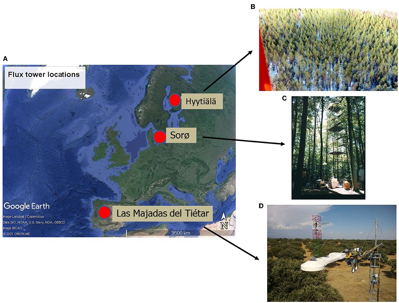
Figure 1. Location of the three European ecosystems (A): Evergreen needle leaf forest of Finland (ENF_FI) (B), Deciduous Broadleaf Forest of Denmark (DBF_DK) (C) and Mediterranean dehesa of Spain (SAV_SP) (D). Images from CEAM (2021) and Fluxnet (2021). Map in (A) from © Google Earth (Landsat/Copernicus).

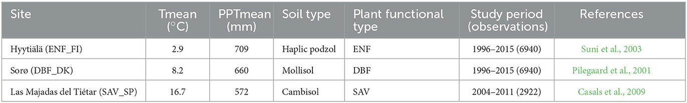
Table 1. Site characteristics of the three flux tower sites (Tmean: mean annual temperature in °C, PPT mean: mean annual rainfall in mm).

The second one, known as Sorø, is located in the east of Denmark at 110 38' 40.7” E and 550 29' 9.1” N at an altitude of 40 m above sea level. It is a Deciduous Broadleaf Forest (DBF_DK) dominated by the European beech (Fagus sylvatica L.), with small scattered stands of Norway spruce (Picea abies L. Karst.), as well as single trees of other conifers such as European larch (Larix decidua Mill.). The climate at this site is temperate maritime with a mean annual temperature of 8.2°C and a mean annual precipitation of 660 mm. The soils are brown soils classified as either Alfisols or Mollisols with a 10–40 cm deep organic layer (Pilegaard et al., 2011).

The third one is known as Las Majadas del Tiétar located in the west of Spain (SAV_SP) at 5°46'29”W and 39°56'26” N at an altitude of ~260 m above sea level. It is Savannah Mediterranean Forest (SAV) known in Spanish as dehesa and is dominated by sclerophyllous holm oaks (Quercus ilex L. ssp. ballota (Desf.) Samp.), with an understory in which Mediterranean grassland species predominate. The climate at this site has typical Mediterranean characteristics with a mean annual temperature of 16.7°C and a mean annual rainfall of 572 mm, with a marked seasonality. The soil is classified as Dystric Cambisol (Casals et al., 2009).

2.2. Flux tower data

In each site, there is an eddy covariance flux tower. The flux towers of Hyytiälä (ENF_FI) and Sorø (DBF_DK) are integrated into the global network FLUXNET (https://fluxnet.fluxdata.org/), and the tower of Las Majadas (SAV_SP) is integrated into the European fluxnet database cluster (https://www.europe-fluxdata.eu/).

The study period of Hyytiälä and Sorø was from 1996 to 2015 and from 2004 to 2011 in Las Majadas. The following pre-processed daily variables for gap-filling and filtering (Papale and Valentini, 2003; Reichstein et al., 2005; Papale et al., 2006) were used (Table 2) as follows: (1) air temperature (Ta, °C), (2) atmospheric pressure (P, hPa), (3) wind speed (WS, m s⁻¹), (4) vapor pressure deficit (VPD, hPa), (5) precipitation (PPT, mm day⁻¹), (6) soil water content (SWC,% vol), (7) latent heat flux (LE, W m⁻²), (8) sensible heat flux (H, W m⁻²), and (9) gross primary productivity (GPP, g C m⁻² day⁻¹).

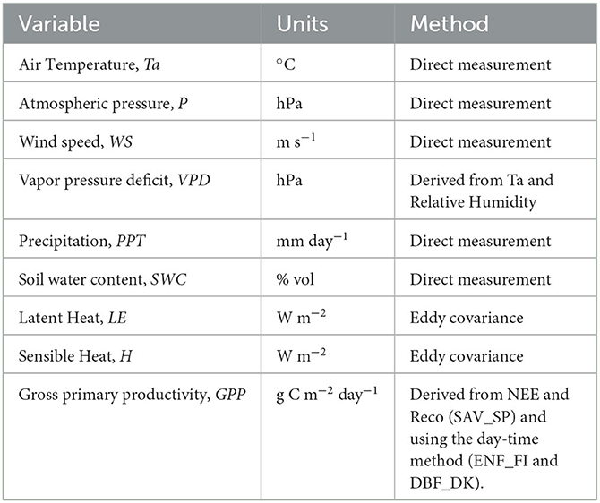
Table 2. Variables obtained from the flux tower sites.

Atmospheric pressure was used to estimate the mixing ratio (r, g H20 kg dry air⁻¹) as follows:

where ε is the ratio of molar masses of vapor and dry air (622), e is the vapor pressure derived from the difference between e_s (the saturation vapor pressure derived from Clausius–Clapeyron equation) and VPD, and P is the atmospheric pressure.

Carbon (net ecosystem exchange) and energy (sensible and latent heat) fluxes were estimated through the eddy covariance method (Baldocchi, 2003, 2014). In ENF_FI and DBF_DK, GPP was calculated according to the daytime method (Lasslop et al., 2010), while in SAV_SP, GPP was calculated as the difference between the ecosystem respiration (Reco, g C m⁻² day⁻¹), which was estimated according to the short-term temperature response of night-time fluxes (Papale and Valentini, 2003; Reichstein et al., 2005) and net ecosystem exchange (NEE, g C m⁻² day⁻¹) (Equation 2).

2.3. Statistical methods

First, all variables were analyzed through a univariate time series analysis. Buys-Ballot tables (Buys-Ballot, 1847), i.e., an average year, were used to study the intra-annual variability of meteorological data, energy fluxes, and GPP. The autocorrelation function was applied to assess the dynamics of the variables' time series allowing the identification of repetitive patterns, periodicity components, and temporal dependency in the time series by a set of correlation coefficients that quantify the relationship between observations at different time intervals (lags) (Box et al., 2015). In our case, our lags correspond to a daily frequency.

Second, the causality of GPP and energy fluxes was studied with Granger causality tests (Granger, 1969), using the alternative tests introduced by Geweke (1984). According to Granger (1969), “… Yt is causing Xt (Yt → Xt) if we are better able to predict Xt using all available information than if the information apart from Yt had been used”. Thus, the Granger causality tests are used to verify the usefulness of one variable to forecast another. The hypothesis of the test is as follows:

The null hypothesis (H0): “past values (at different lags, in our case daily lags) of a variable Yt cannot help to predict other variable Xt”.

The alternative hypothesis (H1): “past values (at different lags, in our case daily lags) of a variable Yt can help to predict other variable Xt”.

The test is based on the following ordinary least squares (OLS) regression model:

where α_j and β_j are the regression coefficients, and ε_t is the error term. Thus, the test is based on the null hypothesis as follows:

H0: β₁ = β₂ = … = β_m = 0 (m =lags)

If we estimate the following restricted equation also by OLS:

Then, the statistic used for the test is an F-statistic based on comparing the sum of square residuals of both models as follows:

Being:

The statistical analysis was computed through Statgraphics 18 (StatPoint Technologies Inc., VA, United States), Eviews 10 University edition (IHS Global Inc., CA, United States), and SAS software (SAS 9.4 Software, SAS Institute Inc., NC, United States).

3. Results

3.1. Average annual patterns of the variables

Figure 2 shows the average annual time series of the three GPP (daily values), i.e., Buys-Ballot. The DBF of Denmark (GPP_DK) and the ENF of Finland (GPP_FI) showed a clear annual cycle with maximum values in June (~16 g C m⁻² day⁻¹) and July (~9 g C m⁻² day⁻¹), respectively, and minimum values close to 0 g C m⁻² day⁻¹ in winter. On the other hand, daily GPP in the dehesa of Spain (GPP_SP) showed minimum values at the end of the summer (~1 g C m⁻² day⁻¹) and winter (~2 g C m⁻² day⁻¹), and maximum values in spring (~7 g C m⁻² day⁻¹) and late autumn (~2 g C m⁻² day⁻¹).

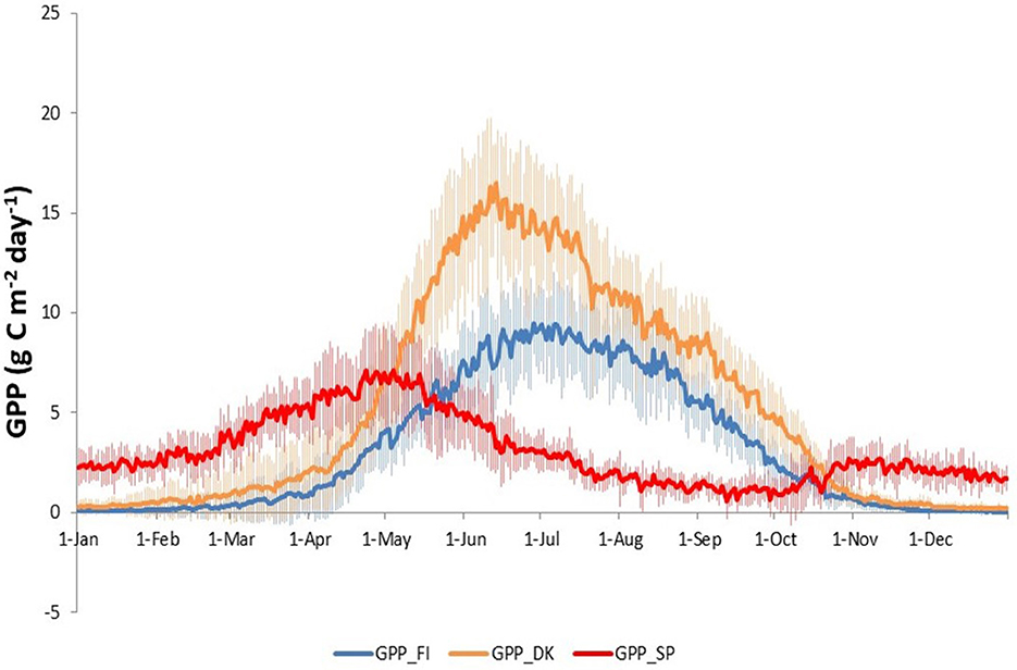
Figure 2. Annual average, i.e., Buys-Ballot, of daily GPP time series in three European ecosystems: Evergreen Needleleaf Forest of Finland (ENF_FI, blue line), Deciduous Broadleaf Forest of Denmark (DBF_DK, orange line) and Mediterranean Savanna ecosystem of Spain (SAV_SP, red line).

Gross primary production (GPP) in Finland and Denmark showed an accumulated annual value of ~1,175 and 1,940 g C m⁻² year⁻¹, respectively, throughout the study period while GPP in Spain exhibited an average annual value of ~1,120 g C m⁻² year⁻¹.

Figure 3 shows the intra-annual dynamics of meteorological variables and energy fluxes for the three ecosystems.

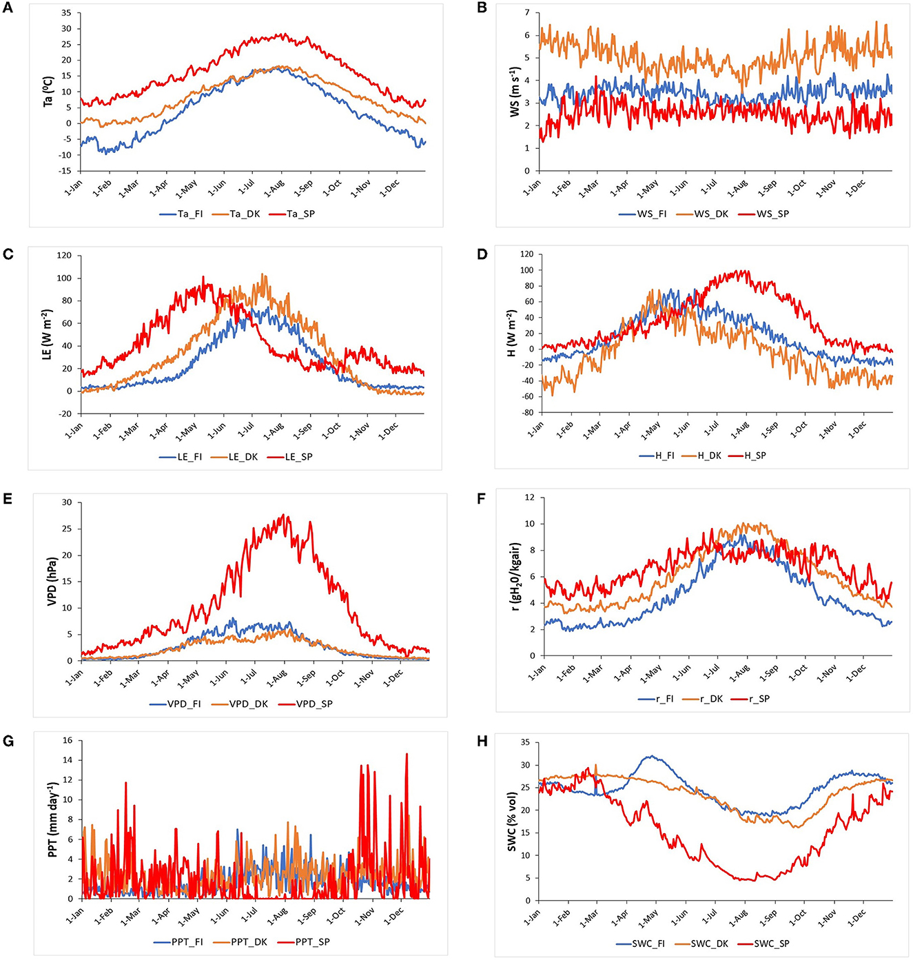
Figure 3. An average year, i.e., Buys-Ballot, of the daily meteorological and energy fluxes variables for the study period in the three European ecosystems [Evergreen Needleleaf Forest of Finland (ENF_FI, blue line), Deciduous Broadleaf Forest of Denmark (DBF_DK, orange line), and Mediterranean Savanna ecosystem of Spain (SAV_SP, red line)]: (A) Air temperature, Ta (°C), (B) Wind speed, WS (m s⁻¹), (C) Latent heat flux, LE (W m⁻²), (D) Sensible heat flux, H (W m⁻²), (E) Vapor pressure deficit, VPD (hPa), (F) Mixing ratio, r (g kg⁻¹) (G) Precipitation, PPT (mm day⁻¹), and (H) Soil water content, SWC (% vol).

The Evergreen Needleleaf Forest of Finland, in a boreal climate, showed minimum values of air temperature (below −5°C) and precipitation (~1.5 mm day⁻¹) during winter and maximum values of both variables in summer (~17°C and 5.5 mm day⁻¹). SWC was relatively constant (~25%) during winter but had a maximum at the end of April after snow melt and a minimum (~20%) during summer, with the maxima temperature and GPP directly related to the evapotranspiration, although PPT was also higher during this season. The wind speed was ~3.5 m s⁻¹ all year, except in summer which had lower values of ~3 m s⁻¹. Due to the low temperatures, LE, VPD, GPP (the three are close to zero), H (~-12 W m⁻²), and r (~2 g kg⁻¹) were minimum during winter. In spring, all these variables increased, especially sensible heat which reached its maximum in mid-May (H~76 W m⁻²). Then, the rest of the variables presented their maxima in summer (Ta~17°C, VPD~8 hPa, LE~75 W m⁻², and r~8.5 g kg⁻¹). Subsequently, they began to decrease at the end of summer and during autumn.

The Deciduous Broadleaf Forest of Denmark is located in a temperate climate and had minimum Ta values in winter (higher than 0°C), and PPT values were relatively constant all year. As a consequence, VPD (~0.5 hPa), LE (~0 W m⁻²), H (~-45 W m⁻²), and r (~4 g kg⁻¹) were also low during winter. Ta began to increase at the end of March, as also happened in Finland; later VPD, LE, and r increased at the same time as GPP did, reaching their maximum values around mid-July (Ta ~ 18°C, VPD ~ 6 hPa, LE ~ 105 W m⁻² and r~10 g kg⁻¹). H also increased from March, but its maximum value (H~75 W m⁻²) was reached in May. At the end of summer, all variables began to decrease (H begin to decrease earlier) and continued decreasing during autumn. Wind speed was higher than in Finland, ~5.8 m s⁻¹ during autumn and winter and ~4.5 m s⁻¹ in spring and summer.

The savanna ecosystem of Spain, located in a Mediterranean climate, is characterized by higher temperatures (~27°C) and a strong drought during summer (PPT ~0 mm day⁻¹, SWC around 5%). Ta was also at its minimum during winter (higher than 5°C), and subsequently, VPD, r, LE, and H were also low during winter (VPD~1.5 hPa, r~6 g kg⁻¹, LE~15 W m⁻², and H~6 W m⁻²). Ta began to increase earlier than in Finland and Denmark, in early March. At the same time, GPP, r, LE, and H also began to increase. LE reached its maximum at the end of April (LE~95 W m⁻²), before the maximum of r which occurred in mid-June (r~8.5 g kg⁻¹) and those of VPD and H occurred at the end of July (VPD~28 hPa, H~100 W m⁻²). At the end of the summer, LE reached its minimum (LE~14 W m⁻²) and then showed a recovery and a second maximum in autumn (LE~40 W m⁻²) directly related to the behavior shown in GPP in Figure 2 and in accordance with the marked seasonality in water availability. Wind speed was ~2.5 m s⁻¹ all year, except in winter which had lower values of ~2 m s⁻¹.

3.2. Assessment of the variable's dynamics

The autocorrelation function (ACF) of the daily GPP had a clear annual pattern in the three ecosystems (Figure 4). The absolute values of GPP_DK and GPP_FI were higher than those of GPP_SP in all lags, with the greatest differences being observed at 180 lags, ~6 months, in the case of negative values. Moreover, GPP_SP showed lower autocorrelation values at the annual lags (lags 365, 730), with less significant values after the second year.

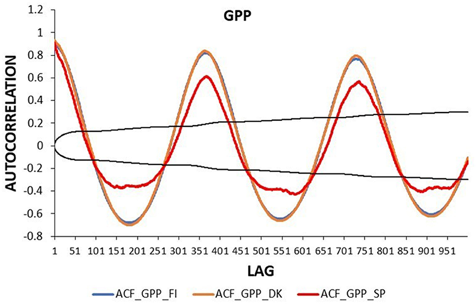
Figure 4. Autocorrelation function of daily GPP time series in three European ecosystems: Evergreen Needleleaf Forest of Finland (ENF_FI, blue line), Deciduous Broadleaf Forest of Denmark (DBF_DK, orange line), and Mediterranean Savanna ecosystem of Spain (SAV_SP, red line). The black lines represent the interval of confidence in the autocorrelation function.

The autocorrelation function for daily meteorological variables and energy fluxes in the three ecosystems is presented in Figure 5. All variables showed a clear annual pattern in the three ecosystems, i.e., the same pattern was found every 365 lags. While in the ENF_FI and DBF_DK, autocorrelation values of the variables at 1 year term were similar to those at the second year term, in Spain they were lower, i.e., lower memory at the long term. The autocorrelation values of Ta were very similar in the three ecosystems at all lags. VPD in the savanna of Spain showed higher ACF values at short, medium, and annual terms than the ENF_FI and the DBF_DK which had similar values. H showed higher ACF values in Spain than in Finland in a short term. However, ACF values in Finland were similar to those in Spain at an annual term (lag 365) and higher at a second-year term (lag 730). Denmark presented the lowest values during all lags. The mixing ratio, r, showed higher ACF values in Finland and Denmark than in Spain during all lags, indicating a higher seasonality. Although very similar values of the ACF of LE were obtained in the three ecosystems in the short term, those of the annual lags of Denmark and Finland were greater than those of Spain. In the three ecosystems, PPT and WS only showed significant values of the ACF in the short term. Although ACF values were lower and not significant, an annual pattern is suggested in the three ecosystems. SWC showed the strongest differences between the three ecosystems. While in Spain, ACF values of SWC revealed a clear annual pattern, values in Finland suggested the presence of two cycles, and in Denmark showed a less marked annual cycle.

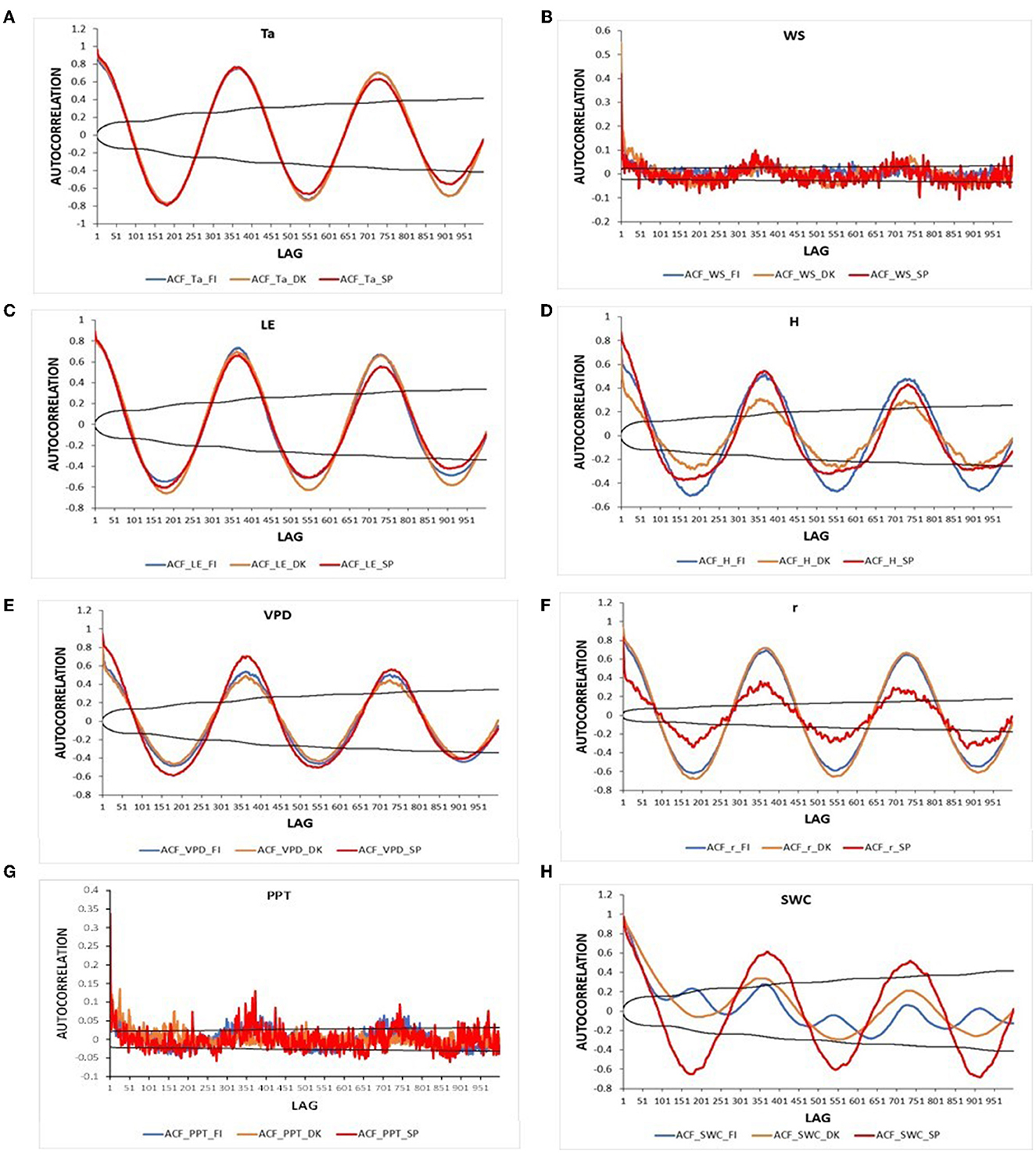
Figure 5. Autocorrelation of the daily meteorological and energy fluxes variables for the study period in the three European ecosystems [Evergreen Needleleaf Forest of Finland (ENF_FI, blue line), Deciduous Broadleaf Forest of Denmark (DBF_DK, orange line), and Mediterranean Savanna ecosystem of Spain (SAV_SP, red line)]: (A) Air temperature (Ta) (°C), (B) Wind speed (WS) (m s⁻¹), (C) Latent heat flux (LE) (W m⁻²), (D) Sensible heat flux (H) (W m⁻²), (E) Vapor pressure deficit (VPD) (hPa), (F) Mixing ratio (r) (g kg⁻¹) (G) Precipitation (PPT) (mm day⁻¹), and (H) Soil water content (SWC) (% vol). The black lines represent the interval of confidence in the autocorrelation values.

3.3. Energy partitioning during the growing period

Figure 6 shows the Bowen ratio (β=H/LE) (a), the ratio between GPP vs. the sum of sensible heat and latent heat (b), the ratio between GPP and sensible heat (c), and the ratio between GPP and latent heat (d), for daily values of the average year during the growing period (April to October for the northern ecosystems and all year for the savanna ecosystem). This period was chosen to select the period when potential solar radiation and temperature were high, avoiding unusual values in these ratios (Wilson et al., 2002).

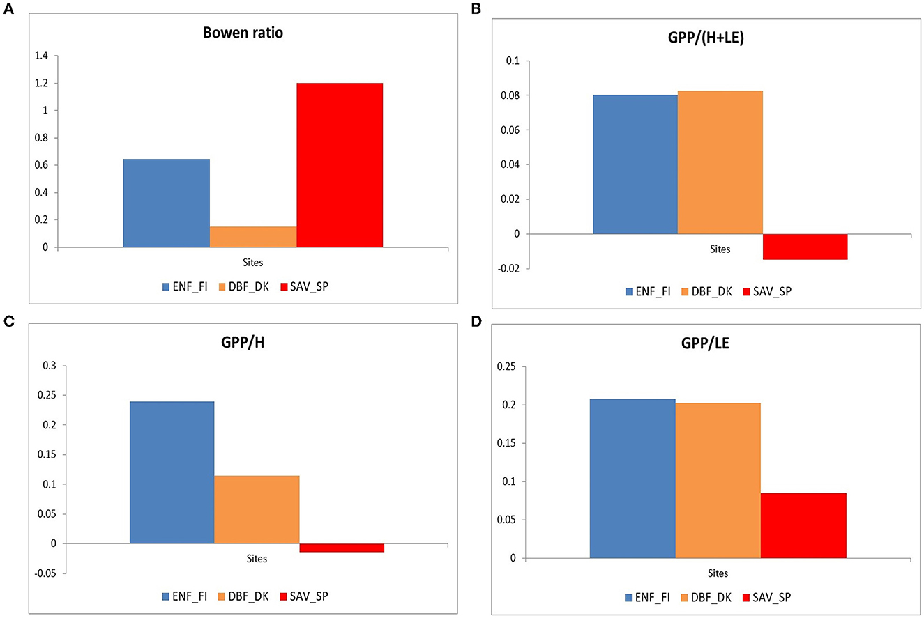
Figure 6. Bowen ratio (A), the ratio between GPP vs. the sum of sensible heat and latent heat (B), the ratio between GPP and sensible heat (C), and the ratio between GPP and latent heat (D) for the three European ecosystems (Evergreen Needleleaf Forest of Finland (ENF_FI, blue), Deciduous Broadleaf Forest of Denmark (DBF_DK, orange), and Mediterranean Savanna ecosystem of Spain (SAV_SP, red) during the growing period (April to October for the northern ecosystems and all year for the savanna ecosystem).

The savanna ecosystem showed the highest Bowen ratio and the lowest calculated ratio. Mediterranean ecosystems present higher radiation and a larger amount of H+LE, which is associated with a lower primary production efficiency in terms of total energy (GPP/(H+LE), panel b), and in terms of sensible heat flux (GPP/H, panel c), with practically null ratios and that could even become negative due to anomalous values in the average year, especially in winter. The evapotranspiration efficiency was also low (GPP/LE, panel d).

On the contrary, both northern ecosystems showed similar production efficiencies in terms of total energy (GPP/(H+LE), panel b) and evapotranspiration (GPP/LE, panel d). However, the Deciduous Broadleaf Forest of Denmark showed a lower Bowen ratio, which leads to a lower GPP/H ratio. This is related to a larger amount of latent heat in relation to sensible heat in DBF_DK and is associated with the larger plant activity in this forest.

3.4. Granger causality tests between GPP and energy fluxes

Figure 7 shows the results of the Granger causality tests between GPP and LE in both directions (GPP⇌LE) and between GPP and H in both directions (GPP⇌H), with the null hypothesis (H0): “the left-side variable does not Granger-cause the right-side variable.”

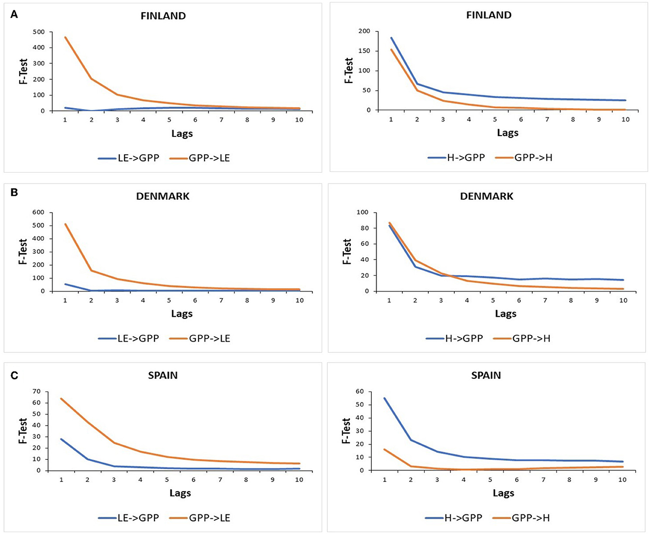
Figure 7. Granger causality tests between GPP, LE, and H in both directions (i.e., energy flux variable cause GPP and GPP cause energy flux variable) for (A) the Evergreen Needleleaf Forest of Finland (ENF_FI), (B) the Deciduous Broadleaf Forest of Denmark (DBF_DK), and (C) the Mediterranean forest of Spain (SAV_SP). Critical values for F-statistic at 0.05 significance level: lag 1 = 3.84, lag 2 = 3.00, lag 3 = 2.60, lag 4 = 2.37, lag 5 = 2.21, lag 6 = 2.10, lag7 = 2.01, lag 8 = 1.94, lag 9 = 1.88, and lag10 = 1.83.

Significant F-test statistics were found when LE caused GPP in the three ecosystems for the first lag, and then values decreased for the following lags. In Finland, F-test values were higher than in Denmark. While in both ecosystems, F-test statistics were significant until lag 10 (except for lag 2 in Finland), and in Spain, F-test statistics were not significant at a 5% confidence level from lag 6 to lag 10.

Significant and higher F-test statistics were found when GPP caused LE in the three ecosystems, especially in Denmark and Finland with very high F-test values decreasing from ~500 for the first lag to 30 in lag 6 but having significant values until lag 10. In Spain, F-test values also showed a decreasing trend but with much lower values ranging approximately between 63 in the first lag and 6 in lag 10.

Significant and higher F-test statistics were found when H caused GPP than in the opposite direction in Finland and Spain. In fact, when GPP caused H in Spain, F-test statistics were only significant at a 5% confidence level for the first two lags. In this sense, H caused GPP and F-test values were higher in Finland than in Spain and showed a decreasing trend from lag 1 to lag 10. Meanwhile, in Denmark, higher F-test statistics were found when GPP caused H at a very short term (3 lags). Then, H caused slightly more GPP than backward.

4. Discussion

The analyses presented served to quantify the importance of the amount of carbon fixed every year by these different types of ecosystems (Beer et al., 2010; Pan et al., 2011), and the results, in terms of the quantity of annual GPP, were consistent with other studies. Lagergren et al. (2008) showed a GPP mean annual value of ~1,612 g C m⁻² year⁻¹ in Denmark and 1,047 g C m⁻² year⁻¹ in Finland at the same flux tower sites for the period between 2000 and 2005, while Cicuéndez et al. (2015) showed an average annual value ~1,091 g C m⁻² year⁻¹ for the 2004–2008 period in the savanna of Spain. In terms of memory, i.e., autocorrelation values in the Mediterranean ecosystem due to the inter-annual variability in SWC which is responsible for the variability in gross primary production and which, in fact, is modulating the variability of LE and r, the two latter variables had less memory at long term than in Finland and Denmark. In contrast, due to very high VPD and H values every summer, the autocorrelation function revealed a more marked annual cycle in these variables than in temperate and boreal climates.

Different patterns in the annual dynamics of the energy partitioning into sensible and latent heat were found between the three sites. In the northern sites (ENF_FI and DBF_DK), most of the available energy was converted into sensible heat at the beginning of the spring, while in the Mediterranean Savanna ecosystem (SAV_SP), this component was dominant in summer, after the growing period (Figure 3). At higher latitudes, low temperatures which caused low VPD values and the lack of vegetative activity resulted in all the energy dedicated to sensible heat, whose maximum was reached before the maximum of temperature and solar radiation. This large sensible heat component had a significant effect on temperature increase that enhanced the beginning of photosynthetic activity and therefore GPP. This has been confirmed by the Granger causality tests which showed that H is statistically causing GPP in both ecosystems (ENF_FI and DBF_DK) probably through its effect on temperature. In fact, the ENF_FI showed a higher GPP/H ratio indicating that the ecosystem is more efficient when radiation was being spent in raising temperature because when optimal temperature conditions were reached, coniferous trees began to produce. According to Mäkelä et al. (2006), the thermal growing season in this site started between 18 April and 7 May. Regarding the DBF_DK, leaf emergence occurred approximately at the end of April, and leaf expansion lasted ~1 month (Wang et al., 2005). Other researchers have found that temperature and day length were limiting factors in this ecosystem during winter, controlling leaf emergence (Basler and Korner, 2014; Dolschak et al., 2019). It seems that the bud-break of beech could coincide with the maximum of sensible heat (Wilson and Baldocchi, 2000). Probably, the first increment in GPP was caused by the growth of herbaceous and shrub species of the ecosystem which are adapted to grow before the shading of beech leaves (Pilegaard et al., 2001; Brunet et al., 2010; Paul-Limoges et al., 2017). It was also probable that coniferous, which represents 20% of the footprint area (Pilegaard et al., 2001), could begin to fix carbon before beech trees (Pilegaard et al., 2001). After this phase, in both ecosystems (DBF_DK and ENF_FI), an increase in transpiration together with higher VPD values (because of higher temperatures) resulted in large and increasing values of the latent heat component that were shown to be caused in a Granger sense by GPP, with high F-test Granger values. In addition, in Denmark, the expansion of LAI led to more shade on the ground which entailed a reduction of changes in surface temperature and subsequently affected H. Thus, GPP affected H more than backward at a very short term (3 lags).

In northern ecosystems, the net radiation continued increasing during the summer, and they are adapted to have the maximum GPP when solar radiation is maximum taking advantage of the optimal conditions for photosynthetic activity and showing clearly higher values of GPP during this period than the water-limited ecosystems (SAV_SP). In fact, tracheid production in coniferous at boreal sites (ENF_FI) occurred around the time of maximum day length and not during the maximum temperature period (Rossi et al., 2006; Kulmala et al., 2017). This fact could explain the delay between the maximum GPP at the end of June, and the maximum temperature, LE, and r at the end of July. However, GPP remained approximately high and constant during summer. In contrast, in DBF_DK, GPP reached a clear maximum at the end of June remaining relatively high for 1 month when LE reached its maximum, with high transpiration rates (Wang et al., 2019), and then began to decrease clearly by the end of July.

However, in the savanna ecosystem of Spain, the temperature was limited only during a short period in winter, and in general the tree and the herbaceous layer could produce during this season (Chiarielllo, 1989; Xu and Baldocchi, 2004; Ma et al., 2007); then, as soon as water was available, the energy was converted into the latent heat component. Water availability is the main limiting factor in this type of ecosystem (Ross et al., 2012; Gilabert et al., 2015; Gómez-Giráldez et al., 2018). In this respect, Jung et al. (2011) showed the importance of the water cycle in the inter-annual carbon fluxes dynamics in semiarid regions. Therefore, in spring, the latent heat was maximum before the maximum temperature and solar radiation. Sridhar et al. (2019) showed this evolution in other semiarid regions. Vegetation in Mediterranean ecosystems, especially grasslands, is adapted to grow earlier in the spring to take advantage of lower temperatures, lower VPD, and higher SWC than the following months (Evans and Young, 1989; Milla et al., 2010; Cicuéndez et al., 2015; Román-Cascón et al., 2020). During this period, GPP was strongly coupled to latent heat and SWC. Thus, Granger causality tests indicated that GPP statistically caused latent heat in the savanna ecosystem, especially due to the GPP of the herbaceous layer which contributes more to the latent heat than the tree layer during spring (El-Madany et al., 2018), especially in savanna ecosystem with a low tree cover. However, F-test values were lower than in the energy-limited regions because the savanna showed lower GPP values, with a lower LAI and less soil water content, and subsequently lower evapotranspiration rates. In summer, the sensible heat was at its maximum, producing high temperatures, while the latent heat reached its minimum values due to the decrease in GPP and the evapotranspiration rate of the species of the herbaceous layer which dried quickly due to high Ta and VPD values. The tree layer can continue to produce a slightly longer period than the herbaceous one because its deeper roots can draw water from the deeper layers of the soil (Joffre and Rambal, 1988; Cubera and Moreno, 2007; Pereira et al., 2007), although during the summer, the stomata will close due to the high VPD and ETP values associated with very high temperatures and lower values of SWC. In addition, the mixing ratio decreased also during summer reaching lower values than in the ENF_FI and DBF_DK.

After summer, in the DBF_DK and the ENF_FI, the net radiation became lower and sensible heat decreased, leading to a decrease in temperature which entailed a reduction in the GPP and the evapotranspiration process, causing a sharp decrease also in latent heat. This period coincided with the browning and fall of leaves in Denmark and the end of the growing season in the coniferous forest of Finland. Then, in winter, sensible heat became even more negative, this fact is related to the higher atmospheric stability conditions reached with cold air trapped close to the surface, and latent heat was nearly zero due to null photosynthetic activity with null GPP values. In addition, in these northern ecosystems, the mixing ratio was much lower than in mid-latitude areas due to their low temperatures that cause air masses with much less contribution to evaporation owing to their high relative humidity. On the other hand, in SAV_SP, during autumn, owing to rainfall events and the recovery of the soil water content, GPP increased (Cicuéndez et al., 2015; El-Madany et al., 2018), and subsequently, the latent heat also showed this recovery, leading to reduce sensible heat, which also decreased owing to less solar heating of the surface. Therefore, in this ecosystem, the latent heat was closely linked to an increase in soil moisture since water is limiting for plants. Thus, in other studies, large soil moisture–latent heat correlations were usually found (Román-Cascón et al., 2021), indicating a stronger land–atmosphere coupling in these transitional zones (Ferguson et al., 2012).

The northern ecosystems are more efficient in terms of water and energy (lower Bowen ratio, higher water use efficiency (GPP/LE), higher GPP/(H+LE), and higher GPP/H) (Figure 6). Although northern ecosystems showed similar ratios, it has to be remarked that during the growing season, the coniferous forest of Finland showed higher net radiation due to a lower albedo and a higher Bowen ratio than the deciduous forest due to higher surface resistance of leaves of coniferous trees and that evaporation is closer to equilibrium at deciduous forests (Wilson et al., 2002; Román-Cascón et al., 2020). Hoek van Dijke et al. (2020) suggested that using the LAI to model or extrapolate surface fluxes of water and energy is possible in savannas, grasslands, and Evergreen Broadleaf Forests, but it is limited in DBF and ENF. It seems that using GPP instead of LAI could improve the results in these ecosystems. This study is a first step to compare the influence of vegetation on the energy fluxes partitioning in clearly contrasted ecosystems located in different climates. However, this study should be extended to similar ecosystems in other areas to obtain more robust conclusions. In addition, it will be interesting to study other types of ecosystems to compare and obtain new results. In terms of energy partitioning, the role of soil heat flux (G) in these ecosystems should also be studied, although it is quite smaller in proportion to latent and sensible fluxes, it may have an effect during the growing season (results not shown).

5. Conclusion

Differences in gross primary production, and latent and sensible heat fluxes at the three different ecosystems analyzed were due to different plant functional types and their interaction with the meteorological variables in each climate. Temperature and solar radiation were the main limiting factors in the northern ecosystems, while water availability was a determinant of growth in the Mediterranean ecosystem. Northern ecosystems were more efficient in terms of water and energy during the growing period (lower Bowen ratio, higher water use efficiency, and higher GPP/H) than Mediterranean ecosystems.

The GPP of the three ecosystems showed a dynamic relationship with the energy fluxes partitioning and water fluxes dynamics confirming that GPP could be used also as a proxy of the influence of vegetation on surface fluxes. In the northern sites, most of the available energy was converted into sensible heat at the beginning of the spring, while in the Mediterranean ecosystems, this component was dominant after the growing period. Meanwhile, in the conifer forests of Finland, the latent heat flux was coupled to GPP during all growing seasons due to the factor of temperature, while in Denmark it began to be strongly coupled when leaf emergence occurred. In Spain, latent heat flux was coupled to GPP during all growing seasons but due to water availability.

The different vegetation types analyzed provide feedback to the atmosphere, influencing the energy partitioning (latent heat and sensible heat fluxes) in a different way. Granger causality tests indicated that GPP was causing latent heat more strongly in the northern ecosystems than in the savanna ecosystem, due to higher LAIs with higher soil water content, which entailed more transpiration rates, especially in the Deciduous Forest. However, sensible heat flux statically causes GPP more than backward, especially in Finland and Spain due to the fact that temperature regulated the carbon fluxes but with an inverse pattern in both ecosystems. In Denmark, a forest with a more closed canopy, the expansion of LAI led to more shade on the ground which entailed a reduction of changes in surface temperature and subsequently affected H among other factors. It is well known that it is essential to include vegetation dynamics to improve atmospheric models. This study is the first step to quantify the intensity and the dominant direction of feedback processes between the ecosystem and the atmospheric boundary layer in different forests, especially focusing on the turbulent heat fluxes (LE and H).

Data availability statement

The original contributions presented in the study are included in the article/supplementary material, further inquiries can be directed to the corresponding authors.

Author contributions

VC, JL, and AP-O: conceptualization. VC, JL, VS-G, LR, and CS: methodology. JL and AP-O: software and resources. VC, JL, and VS-G: formal analysis. VC, JL, VS-G, CR-C, CY, and AP-O: investigation. VC, CR-C, CY, and AP-O: writing—original draft preparation. VC, CR-C, LR, CS, CY, and AP-O: writing—review and editing. AP-O: supervision. CY and AP-O: funding acquisition. All authors have read and agreed to the published version of the manuscript.

Funding

This research was conducted in the framework of the I+D+i Spanish National Projects AGL-2010-17505, the PID2020-115509RB-I00 project (INFOLANDYN), and the PID2020-115321RB-I00 project (LATMOS-i) funded by the Ministerio de Ciencia e Innovación of Spain MCIN/AEI/ 10.13039/501100011033. VC was supported by a post-doctoral Juan de la Cierva fellowship (FJC2021-046735-I) funded by the Spanish Ministerio de Ciencia e Innovación MCIN/AEI/ 10.13039/501100011033 and by the European Union ≪NextGenerationEU≫/PRTR≫. LR was supported by a UPM grant as part of the national research program Recualificación del Sistema Universitario Español, financed by the Recovery and Resilience Package—NextGenerationEU (European Commission). CS was also supported by a predoctoral scholarship awarded by the Community of Madrid (No. IND2020/AMB-17747).

Acknowledgments

We would like to thank the FLUXNET2015 data set and the European Fluxes Database Cluster for the permission to download the data of the three flux towers. The authors would like to thank the head researchers of the flux towers.

Conflict of interest

The authors declare that the research was conducted in the absence of any commercial or financial relationships that could be construed as a potential conflict of interest.

Publisher's note

All claims expressed in this article are solely those of the authors and do not necessarily represent those of their affiliated organizations, or those of the publisher, the editors and the reviewers. Any product that may be evaluated in this article, or claim that may be made by its manufacturer, is not guaranteed or endorsed by the publisher.

References

Arora, V. (2002). Modeling vegetation as a dynamic component in soil-vegetation-atmosphere transfer schemes and hydrological models. Rev. Geophys. 40, 1006. doi: 10.1029/2001RG000103
Aubinet, M., Vesala, T., and Papale, D. (2012). Eddy Covariance: A Practical Guide to Measurement and Data Analysis. Dordrecht: Springer Netherlands. doi: 10.1007/978-94-007-2351-1
Baldocchi, D. (2014). Measuring fluxes of trace gases and energy between ecosystems and the atmosphere—the state and future of the eddy covariance method. Glob. Chang. Biol. 20, 3600–3609. doi: 10.1111/gcb.12649
Baldocchi, D., Falge, E., Gu, L., Olson, R., Hollinger, D., Running, S., et al. (2001a). FLUXNET: a new tool to study the temporal and spatial variability of ecosystem-scale carbon dioxide, water vapor, and energy flux densities. Bull. Am. Meteorol. Soc. 82, 2415–2434. doi: 10.1175/1520-0477(2001)082<2415:FANTTS>2.3.CO;2
Baldocchi, D., Falge, E., and Wilson, K. (2001b). A spectral analysis of biosphere–atmosphere trace gas flux densities and meteorological variables across hour to multi-year time scales. Agricult. Forest Meteorol. 107, 1–27. doi: 10.1016/S0168-1923(00)00228-8
Baldocchi, D. D. (2003). Assessing the eddy covariance technique for evaluating the carbon balance of ecosystems. Glob. Chang. Biol. 9, 1–41. doi: 10.1046/j.1365-2486.2003.00629.x
Baldocchi, D. D., Hincks, B. B., and Meyers, T. P. (1988). Measuring biosphere-atmosphere exchanges of biologically related gases with micrometeorological methods. Ecology. 69, 1331–1340. doi: 10.2307/1941631
Basler, D., and Korner, C. (2014). Photoperiod and temperature responses of bud swelling and bud burst in four temperate forest tree species. Tree Physiol. 34, 377–388. doi: 10.1093/treephys/tpu021
Beer, C., Reichstein, M., Tomelleri, E., Ciais, P., Jung, M., Carvalhais, N., et al. (2010). Terrestrial gross carbon dioxide uptake: global distribution and covariation with climate. Science 329, 834–838. doi: 10.1126/science.1184984
Box, G. E., Jenkins, G. M., Reinsel, G. C., and Ljung, G. M. (2015). Time Series Analysis: Forecasting and Control. New Jersey: John Wiley and Sons, Inc.
Brunet, J., Fritz, Ö., and Richnau, G. (2010). Biodiversity in European beech forests—a review with recommendations for sustainable forest management. Ecol. Bull. 53, 77–94.
Buys-Ballot, C. H. D. (1847). Les Changements périodiques de température, dépendants de la nature du soleil et de la lune, mis en rapport avec le pronostic du temps, déduits d'observations néerlandaises de 1729 à 1846.' Kemink.
Casals, P., Gimeno, C., Carrara, A., Lopez-Sangil, L., and Sanz, M. J. (2009). Soil CO2 efflux and extractable organic carbon fractions under simulated precipitation events in a Mediterranean Dehesa. Soil Biol. Biochem. 41, 1915–1922. doi: 10.1016/j.soilbio.2009.06.015
CEAM (2021). Available online at: http://ceamflux.com:9090/index.html (accessed May 3, 2021).
Chiarielllo, N. R. (1989). “Phenology of California grasslands,” in Grassland structure and Function: California Annual Grassland (Tasks for Vegetation Science 2.0), eds H. Lieth and H. A. Mooney (Dordrecht, The Netherlands: Kluwer Academic Publishers), p. 47–58. doi: 10.1007/978-94-009-3113-8_5
Ciais, P., Reichstein, M., Viovy, N., Granier, A., Ogée, J., Allard, V., et al. (2005). Europe-wide reduction in primary productivity caused by the heat and drought in 2003. Nature. 437, 529–533. doi: 10.1038/nature03972
Cicuéndez, V., Litago, J., Huesca, M., Rodriguez-Rastrero, M., Recuero, L., Merino-de-Miguel, S., et al. (2015). Assessment of the gross primary production dynamics of a Mediterranean holm oak forest by remote sensing time series analysis. Agroforestry Syst. 89, 491–510. doi: 10.1007/s10457-015-9786-x
Cubera, E., and Moreno, G. (2007). Effect of single quercus ilex trees upon spatial and seasonal changes in soil water content in dehesas of central western Spain. Ann. For. Sci. 64, 355–364. doi: 10.1051/forest:2007012
Detto, M., Bohrer, G., Nietz, J., Maurer, K., Vogel, C., Gough, C., et al. (2013). Multivariate conditional granger causality analysis for lagged response of soil respiration in a temperate forest. Entropy. 15, 4266–4284. doi: 10.3390/e15104266
Dolschak, K., Gartner, K., and Berger, T. W. (2019). The impact of rising temperatures on water balance and phenology of European beech (Fagus sylvatica L.) stands. Model. Earth Syst. Environ. 5, 1347–1363. doi: 10.1007/s40808-019-00602-1
Dornelas, M., Magurran, A. E., Buckland, S. T., Chao, A., Chazdon, R. L., Colwell, R. K., et al. (2013). Quantifying temporal change in biodiversity: challenges and opportunities. Proc. R. Soc. B Biol. Sci. 280, 20121931. doi: 10.1098/rspb.2012.1931
El-Madany, T. S., Reichstein, M., Perez-Priego, O., Carrara, A., Moreno, G., Pilar Martín, M., et al. (2018). Drivers of spatio-temporal variability of carbon dioxide and energy fluxes in a Mediterranean savanna ecosystem. Agric. Forest Meteorol. 262, 258–278. doi: 10.1016/j.agrformet.2018.07.010
Esau, I. N., and Lyons, T. J. (2002). Effect of sharp vegetation boundary on the convective atmospheric boundary layer. Agric. Forest Meteorol. 114, 3–13. doi: 10.1016/S0168-1923(02)00154-5
Evans, R. A., and Young, J. A. (1989). “Characterization and analysis of abiotic factors and their influences on vegetation,” in Grassland Structure and Function: California annual Grassland (Tasks for vegetation science 2, 0.), eds H. Lieth and H. A. Mooney (Dordrecht, The Netherlands: Kluwer Academic Publishers). doi: 10.1007/978-94-009-3113-8_2
Ferguson, C. R., Wood, E. F., and Vinukollu, R. K. (2012). A global intercomparison of modeled and observed land–atmosphere coupling*. J. Hydrometeorol. 13, 749–784. doi: 10.1175/JHM-D-11-0119.1
Fluxnet (2021). Available online at: https://fluxnet.org/ (accessed Mar 5, 2021).
Forzieri, G., Miralles, D. G., Ciais, P., Alkama, R., Ryu, Y., Duveiller, G., et al. (2020). Increased control of vegetation on global terrestrial energy fluxes. Nat. Clim. Chang. 10, 356–362. doi: 10.1038/s41558-020-0717-0
Geweke, J. (1984). “Inference and Causality in Economic Time Series Models,” in Handbook of Econometrics, eds Z. Grilliches and M. D. Intriligator (Amsterdam: Elsevier Science Publisher). doi: 10.1016/S1573-4412(84)02011-0
Gilabert, M. A., Moreno, A., Maselli, F., Martínez, B., Chiesi, M., Sánchez-Ruiz, S., et al. (2015). Daily GPP estimates in Mediterranean ecosystems by combining remote sensing and meteorological data. ISPRS J. Photogrammetry Remote Sens. 102, 184–197. doi: 10.1016/j.isprsjprs.2015.01.017
Gómez-Giráldez, P. J., Carpintero, E., Ramos, M., Aguilar, C., and González-Dugo, M. P. (2018). Effect of the water stress on gross primary production modeling of a Mediterranean oak savanna ecosystem. Proc. Int. Assoc. Hydrol. Sci. 380, 37–43. doi: 10.5194/piahs-380-37-2018
Granger, C. W. J. (1969). Investigating causal relations by econometric models and cross-spectral methods. Econometrica. 37, 424–438. doi: 10.2307/1912791
Hamilton, J. D. (1994). Time Series Analysis. Princeton: Princeton University Press. doi: 10.1515/9780691218632
Hoek van Dijke, A., Mallick, K., Schlerf, M., Machwitz, M., Herold, M., and Teuling, A. (2020). Examining the link between vegetation leaf area and land-atmosphere exchange of water, energy, and carbon fluxes using FLUXNET data. Biogeosci. Discuss. 17, 4443–57. doi: 10.5194/bg-17-4443-2020
Huesca, M., Litago, J., Palacios-Orueta, A., Montes, F., Sebastián-López, A., and Escribano, P. (2009). Assessment of forest fire seasonality using MODIS fire potential: a time series approach. Agric. Forest Meteorol. 149, 1946–1955. doi: 10.1016/j.agrformet.2009.06.022
Huesca, M., Merino-de-Miguel, S., Eklundh, L., Litago, J., Cicuéndez, V., Rodríguez-Rastrero, M., et al. (2015). Ecosystem functional assessment based on the “optical type” concept and self-similarity patterns: an application using MODIS-NDVI time series autocorrelation. Int. J. Appl. Earth Observ. Geoinform. 43, 132–148. doi: 10.1016/j.jag.2015.04.008
Jamiyansharav, K., Ojima, D., Pielke, R. A., Parton, W., Morgan, J., Beltrán-Przekurat, A., et al. (2011). Seasonal and interannual variability in surface energy partitioning and vegetation cover with grazing at shortgrass steppe. J. Arid Environ. 75, 360–370. doi: 10.1016/j.jaridenv.2010.11.008
Jiang, B., Liang, S., and Yuan, W. (2015). Observational evidence for impacts of vegetation change on local surface climate over northern China using the Granger causality test. J. Geophys. Res. Biogeosci. 120, 1–12. doi: 10.1002/2014JG002741
Joffre, R., and Rambal, S. (1988). Soil water improvement by trees in the rangelands of southern Spain. Acta oecologica. Oecologia plantarum 9, 405–422.
Jung, M., Reichstein, M., Margolis, H. A., Cescatti, A., Richardson, A. D., Arain, M. A., et al. (2011). Global patterns of land-atmosphere fluxes of carbon dioxide, latent heat, and sensible heat derived from eddy covariance, satellite, and meteorological observations. J. Geophys. Res. 116, G00J.07. doi: 10.1029/2010JG001566
Kang, X., Wang, Y., Chen, H., Tian, J., Cui, X., Rui, Y., et al. (2014). Modeling carbon fluxes using multi-temporal modis imagery and Co2 eddy flux tower data in zoige alpine wetland, south-west China. Wetlands. 34, 603–618. doi: 10.1007/s13157-014-0529-y
Krich, C., Runge, J., Miralles, D. G., Migliavacca, M., Perez-Priego, O., El-Madany, T., et al. (2020). Estimating causal networks in biosphere-atmosphere interaction with the PCMCI approach. Biogeosciences. 17, 1033–1061. doi: 10.5194/bg-17-1033-2020
Kueppers, L. M., Snyder, M. A., and Sloan, L. C. (2007). Irrigation cooling effect: Regional climate forcing by land-use change. Geophys. Res. Lett. 34, L03703. doi: 10.1029/2006GL028679
Kulmala, L., Read, J., Nöjd, P., Rathgeber, C. B. K., Cuny, H. E., Hollmén, J., et al. (2017). Identifying the main drivers for the production and maturation of Scots pine tracheids along a temperature gradient. Agricult. Forest Meteorol. 232, 210–224. doi: 10.1016/j.agrformet.2016.08.012
Lagergren, F., Lindroth, A., Dellwik, E., Ibrom, A., Lankreijer, H., Launiainen, S., et al. (2008). Biophysical controls on CO2 fluxes of three Northern forests based on long-term eddy covariance data. Tellus B Chem. Phys. Meteorol. 60, 143–152. doi: 10.1111/j.1600-0889.2006.00324.x
Lan, X., Li, Y., Shao, R., Chen, X., Lin, K., Cheng, L., et al. (2020). Vegetation controls on surface energy partitioning and water budget over China. J. Hydrol. 600, 125646. doi: 10.1016/j.jhydrol.2020.125646
Lasslop, G., Reichstein, M., Papale, D., Richardson, A. D., Arneth, A., Barr, A., et al. (2010). Separation of net ecosystem exchange into assimilation and respiration using a light response curve approach: critical issues and global evaluation. Glob. Chang. Biol. 16, 187–208. doi: 10.1111/j.1365-2486.2009.02041.x
Lu, Y., and Kueppers, L. M. (2012). Surface energy partitioning over four dominant vegetation types across the United States in a coupled regional climate model (Weather Research and Forecasting Model 3-Community Land Model 3.5). J. Geophys. Res. Atmospheres. 117, 1–14. doi: 10.1029/2011JD016991
Ma, N., Niu, G. Y., Xia, Y., Cai, X., Zhang, Y., Ma, Y., et al. (2017). A systematic evaluation of noah-MP in simulating land-atmosphere energy, water, and carbon exchanges over the continental United States. J. Geophys. Res. Atmospheres. 122, 245–268. doi: 10.1002/2017JD027597
Ma, S., Baldocchi, D. D., Xu, L., and Hehn, T. (2007). Inter-annual variability in carbon dioxide exchange of an oak/grass savanna and open grassland in California. Agricult. Forest Meteorol. 147, 157–171. doi: 10.1016/j.agrformet.2007.07.008
Mäkelä, A., Kolari, P., Karimäki, J., Nikinmaa, E., Perämäki, M., and Hari, P. (2006). Modelling five years of weather-driven variation of GPP in a boreal forest. Agricult. Forest Meteorol. 139, 382–398. doi: 10.1016/j.agrformet.2006.08.017
Malhi, Y., Roberts, J. T., Betts, R. A., Killeen, T. J., Li, W., Nobre, C. A., et al. (2008). Climate change, deforestation, and the fate of the Amazon. Science. 319, 169–172. doi: 10.1126/science.1146961
Milla, R., Castro-Díez, P., and Montserrat-Martí, G. (2010). Phenology of Mediterranean woody plants from NE Spain: Synchrony, seasonality, and relationships among phenophases. Flora Morphol. Distribut. Funct. Ecol. Plants. 205, 190–199. doi: 10.1016/j.flora.2009.01.006
Nemani, R. R., Keeling, C. D., Hashimoto, H., Jolly, W. M., Piper, S. C., Tucker, C. J., et al. (2003). Climate-driven increases in global terrestrial net primary production from 1982 to 1999. Science. 300, 1560–1563. doi: 10.1126/science.1082750
Pan, Y., Birdsey, R. A., Fang, J., Houghton, R., Kauppi, P. E., Kurz, W. A., et al. (2011). A large and persistent carbon sink in the world's forests. Science. 333, 988–993. doi: 10.1126/science.1201609
Papagiannopoulou, C., Miralles, D. G., Decubber, S., Demuzere, M., Verhoest, N. E. C., Dorigo, W. A., et al. (2017). A non-linear Granger-causality framework to investigate climate–vegetation dynamics. Geosci. Model Develop. 10, 1945–1960. doi: 10.5194/gmd-10-1945-2017
Papale, D., Reichstein, M., Aubinet, M., Canfora, E., Bernhofer, C., Kutsch, W., et al. (2006). Towards a standardized processing of Net Ecosystem Exchange measured with eddy covariance technique: algorithms and uncertainty estimation. Biogeosciences. 3, 571–583. doi: 10.5194/bg-3-571-2006
Papale, D., and Valentini, R. (2003). A new assessment of European forests carbon exchanges by eddy fluxes and artificial neural network spatialization. Glob. Chang. Biol. 9, 525–535. doi: 10.1046/j.1365-2486.2003.00609.x
Paul-Limoges, E., Wolf, S., Eugster, W., Hörtnagl, L., and Buchmann, N. (2017). Below-canopy contributions to ecosystem CO2 fluxes in a temperate mixed forest in Switzerland. Agricult. Forest Meteorol. 247, 582–596. doi: 10.1016/j.agrformet.2017.08.011
Pereira, J. S., Mateus, J. A., Aires, L. M., Pita, G., Pio, C., David, J. S., et al. (2007). Net ecosystem carbon exchange in three contrasting Mediterranean ecosystems—the effect of drought. Biogeosciences. 4, 791–802. doi: 10.5194/bg-4-791-2007
Pilegaard, K., Hummelshøj, P., Jensen, N. O., and Chen, Z. (2001). Two years of continuous CO2 eddy-flux measurements over a Danish beech forest. Agricult. Forest Meteorol. 107, 29–41. doi: 10.1016/S0168-1923(00)00227-6
Pilegaard, K., Ibrom, A., Courtney, M. S., Hummelshøj, P., and Jensen, N. O. (2011). Increasing net CO2 uptake by a Danish beech forest during the period from 1996 to 2009. Agricult. Forest Meteorol. 151, 934–946. doi: 10.1016/j.agrformet.2011.02.013
Recuero, L., Wiese, K., Huesca, M., Cicuéndez, V., Litago, J., Tarquis, A. M., et al. (2019). Fallowing temporal patterns assessment in rainfed agricultural areas based on NDVI time series autocorrelation values. Int. J. Appl. Earth Observat. Geoinform. 82, 101890. doi: 10.1016/j.jag.2019.05.023
Reichstein, M., Falge, E., Baldocchi, D., Papale, D., Aubinet, M., Berbigier, P., et al. (2005). On the separation of net ecosystem exchange into assimilation and ecosystem respiration: review and improved algorithm. Glob. Chang. Biol. 11, 1424–1439. doi: 10.1111/j.1365-2486.2005.001002.x
Román-Cascón, C., Lothon, M., Lohou, F., Hartogensis, O., Vila-Guerau de Arellano, J., Pino, D., et al. (2020). Can we use satellite-based soil-moisture products at high resolution to investigate land-use differences and land–atmosphere Interactions? A case study in the savanna. Remote Sens. 12, 1701. doi: 10.3390/rs12111701
Román-Cascón, C., Lothon, M., Lohou, F., Hartogensis, O., Vila-Guerau de Arellano, J., Pino, D., et al. (2021). Surface representation impacts on turbulent heat fluxes in the weather research and forecasting (WRF) model (v.4.1.3). Geosci. Model Develop. 14, 3939–3967. doi: 10.5194/gmd-14-3939-2021
Ross, I., Misson, L., Rambal, S., Arneth, A., Scott, R. L., Carrara, A., et al. (2012). How do variations in the temporal distribution of rainfall events affect ecosystem fluxes in seasonally water-limited Northern Hemisphere shrublands and forests?. Biogeosciences. 9, 1007–1024. doi: 10.5194/bg-9-1007-2012
Rossi, S., Deslauriers, A., Anfodillo, T., Morin, H., Saracino, A., Motta, R., et al. (2006). Conifers in cold environments synchronize maximum growth rate of tree-ring formation with day length. New Phytol. 170, 301–310. doi: 10.1111/j.1469-8137.2006.01660.x
Schimel, D., Pavlick, R., Fisher, J. B., Asner, G. P., Saatchi, S., Townsend, P., et al. (2015). Observing terrestrial ecosystems and the carbon cycle from space. Glob. Chang. Biol. 21, 1762–1776. doi: 10.1111/gcb.12822
Seneviratne, S. I., and Stöckli, R. (2008). “The role of land-atmosphere interactions for climate variability in Europe,” in Climate Variability and Extremes during the Past 100 Years (Dordrecht: Springer Netherlands), p. 179–193. doi: 10.1007/978-1-4020-6766-2_12
Setiawan, Y., Rustiadi, E., Yoshino, K., and Liyantono, Effendi, H. (2014). Assessing the seasonal dynamics of the java's paddy field using MODIS satellite images. ISPRS Int. J. Geo-Inform. 3, 110–129. doi: 10.3390/ijgi3010110
Shukla, P. R., Skeg, J., Calvo Buendia, E., Masson-Delmotte, V., Pörtner, H.-O., Roberts, D. C., et al. (2019). Climate Change and Land: An IPCC Special Report on Climate Change, Desertification, Land Degradation, Sustainable Land Management, Food Security, and Greenhouse Gas Fluxes in Terrestrial Ecosystems. Ginevra, IPCC
Sridhar, V., Billah, M. M., and Valayamkunnath, P. (2019). Field-scale intercomparison analysis of ecosystems in partitioning surface energy balance components in a semi-arid environment. Ecohydrology and Hydrobiology. 19, 24–37. doi: 10.1016/j.ecohyd.2018.06.005
Suni, T., Rinne, J., Reissell, A., Altimir, N., Keronen, P., Rannik, Ü., et al. (2003). Long-term measurements of surface fluxes above a Scots pine forest in Hyytiälä, southern Finland, 1996–2001. Boreal Environ. Res. 8, 287–301.
Tornos, L., Huesca, M., Dominguez, J. A., Moyano, M. C., Cicuendez, V., Recuero, L., et al. (2015). Assessment of MODIS spectral indices for determining rice paddy agricultural practices and hydroperiod. ISPRS J. Photogram. Remote Sens. 101, 110–124. doi: 10.1016/j.isprsjprs.2014.12.006
Wang, P., Li, X., Tong, Y., Huang, Y., Yang, X., and Wu, X. (2019). Vegetation dynamics dominate the energy flux partitioning across typical ecosystem in the Heihe River Basin: observation with numerical modeling. J. Geograph. Sci. 29, 1565–1577. doi: 10.1007/s11442-019-1677-z
Wang, Q., Tenhunen, J., Dihn, N., Reichstein, M., Otieno, D., Granier, A., et al. (2005). Evaluation of seasonal variation of MODIS derived leaf area index at two European deciduous broadleaf forest sites. Remote Sens. Environ. 96, 475–484. doi: 10.1016/j.rse.2005.04.003
Williams, I. N., Lu, Y., Kueppers, L. M., Riley, W. J., Biraud, S. C., Bagley, J. E., et al. (2016). Land-atmosphere coupling and climate prediction over the U.S. southern great plains. J. Geophys. Res. 121, 125–145. doi: 10.1002/2016JD025223
Williams, I. N., and Torn, M. S. (2015). Vegetation controls on surface heat flux partitioning, and land-atmosphere coupling. Geophys. Res. Lett. 42, 9416–9424. doi: 10.1002/2015GL066305
Wilson, K. B., and Baldocchi, D. D. (2000). Seasonal and interannual variability of energy fluxes over a broadleaved temperate deciduous forest in North America. Agricult. Forest Meteorol. 100, 1–18. doi: 10.1016/S0168-1923(99)00088-X
Wilson, K. B., Baldocchi, D. D., Aubinet, M., Berbigier, P., Bernhofer, C., Dolman, H., et al. (2002). Energy partitioning between latent and sensible heat flux during the warm season at FLUXNET sites. Water Resour. Res. 38, 30–1.-30–11. doi: 10.1029/2001WR000989
Keywords: gross primary production, surface energy fluxes, Granger causality, flux tower, autocorrelation function, atmosphere-vegetation feedback, vegetation dynamics
Citation: Cicuéndez V, Litago J, Sánchez-Girón V, Román-Cascón C, Recuero L, Saénz C, Yagüe C and Palacios-Orueta A (2023) Dynamic relationships between gross primary production and energy partitioning in three different ecosystems based on eddy covariance time series analysis. Front. For. Glob. Change 6:1017365. doi: 10.3389/ffgc.2023.1017365
Received: 11 August 2022; Accepted: 27 February 2023;
Published: 20 March 2023.
Edited by:
Eduardo Maeda, University of Helsinki, FinlandReviewed by:
Rita Von Randow, São Paulo State Technological College, BrazilLuis Manuel Navas, University of Valladolid, Spain
Copyright © 2023 Cicuéndez, Litago, Sánchez-Girón, Román-Cascón, Recuero, Saénz, Yagüe and Palacios-Orueta. This is an open-access article distributed under the terms of the Creative Commons Attribution License (CC BY). The use, distribution or reproduction in other forums is permitted, provided the original author(s) and the copyright owner(s) are credited and that the original publication in this journal is cited, in accordance with accepted academic practice. No use, distribution or reproduction is permitted which does not comply with these terms.
*Correspondence: Víctor Cicuéndez, victor.cicuendez.lopezocana@upm.es; Alicia Palacios-Orueta, alicia.palacios@upm.es